2. Tutorial

This tutorial is intended to be read in order. It introduces the available tools of the package in a specific order so that the reader can discover all the features of the package organically.

In the following tutorial, the variable f refers to one or several file paths stored in a vector. It can also be the path to a directory or the path of a virtual point cloud. In this tutorial, the output is rendered with one or two small LAS files, but every pipeline is designed to process numerous files covering a large extent.

Overall functionality

In lasR, the R functions provided to the user are not designed to process the data directly; instead, they are used to create a pipeline. A pipeline consists of stages that are applied to a point cloud in order. Each stage can either transform the point cloud within the pipeline without generating any output or process the point cloud to produce an output.

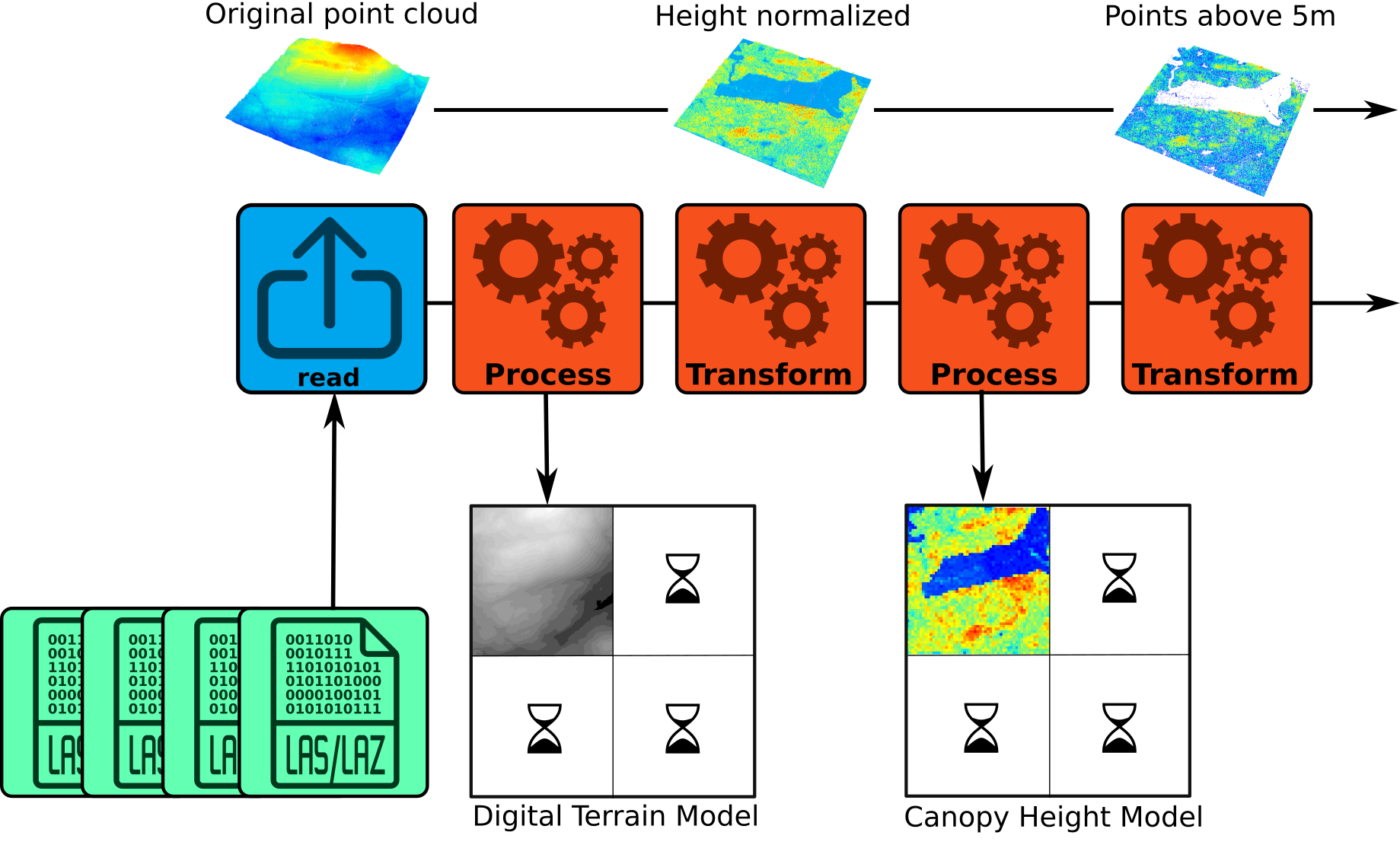
In the figure below, there are 4 LAS/LAZ files and a pipeline that (1) reads a file, (2) builds and writes a DTM on disk, (3) transforms the point cloud by normalizing the elevation, (4) builds a canopy height model using the transformed point cloud, and (5) transforms the point cloud by removing points below 5 m. The resulting version of the point cloud (points above 5m) is discarded and lost because there is no additional stage in this pipeline. However, other stages can be added, such as the application of a predictive model for points above 5 m or a stage that writes the point cloud to disk.

Once the first file completes the entire pipeline, the second file is used, and the pipeline is applied to fill in the missing parts of the geospatial rasters or vectors produced by the pipeline. Each file is loaded with a buffer from neighboring files if needed.

A pipeline created from the R interface does nothing initially. After building the pipeline, users must call the exec() function on it to initiate the computation.

Reader

The reader_las() stage MUST be the first stage of any pipeline (blue in the figure above). It takes as input the list of files to process. When creating a pipeline with only this stage, the header of the files are read, but no computation is actually applied. The points are not even read because there is no other stage in the pipeline that require to read the points. No result is returned.

pipeline = reader_las()
exec(pipeline, on = f)
#> NULL

In practice when using read_las() without argument it can be omitted, the function exec adds it on-the-fly.

Triangulate

The first stage we can try is triangulate(). This algorithm performs a Delaunay triangulation on the points of interest. Triangulating points is a very useful task that is employed in numerous processing tasks. Triangulating all points is not very interesting, so we usually want to use the filter argument to triangulate only specific points of interest.

In the following example, we triangulate the points classified as 2 (i.e., ground). This produces a meshed Digital Terrain Model.

In this example, the files are read sequentially, with points loaded one by one and stored to build a Delaunay triangulation. In lasR, only one file is stored in memory at a time. The program stores the point cloud and the Delaunay triangulation for the current processing file. Then the data are discarded to load a new file.

If the users do not provide a path to an output file to store the result, the result is lost. In the following pipeline, we are building a triangulation of the ground points, but we get no output because everything is lost.

pipeline = reader_las() + triangulate(filter = keep_ground())
ans = exec(pipeline, on = f)
ans
#> NULL

In the following pipeline the triangulation is stored in a geopackage file by providing an argument ofile:

pipeline = reader_las() + triangulate(filter = keep_ground(), ofile = tempgpkg())
ans = exec(pipeline, on = f)
ans
#> Simple feature collection with 1 feature and 0 fields
#> Geometry type: MULTIPOLYGON
#> Dimension:     XYZ
#> Bounding box:  xmin: 273357.2 ymin: 5274357 xmax: 273642.9 ymax: 5274643
#> z_range:       zmin: 788.9932 zmax: 814.8322
#> Projected CRS: NAD83(CSRS) / MTM zone 7
#> # A tibble: 1 × 1
#>                                                                             geom
#>                                                               <MULTIPOLYGON [m]>
#> 1 Z (((273500.4 5274501 808.4787, 273501.2 5274502 808.1748, 273500.4 5274502 8…

par(mar = c(2, 2, 1, 1))
plot(ans, axes = T, lwd = 0.5)

We can also triangulate the first returns. This produce a meshed Digital Surface Model.

read = reader_las()
del = triangulate(filter = keep_first(), ofile = tempgpkg())
ans = exec(read+del, on = f)

We can also perform both triangulations in the same pipeline. The idea of lasR is to execute all the tasks in one pass using a pipeline:

read = reader_las()
del1 = triangulate(filter = keep_ground(), ofile = tempfile(fileext = ".gpkg"))
del2 = triangulate(filter = keep_first(), ofile = tempfile(fileext = ".gpkg"))
pipeline = read + del1 + del2
ans = exec(pipeline, on = f)

Using triangulate() without any other stage in the pipeline is usually not very useful. Typically, triangulate() is employed without the ofile argument as an intermediate step. For instance, it can be used with rasterize().

Rasterize

rasterize() does exactly what users may expect from it and even more. There are three variations:

Rasterize with predefined operators. The operators are optimized internally, making the operations as fast as possible, but the number of registered operators is finite.
Rasterize by injecting a user-defined R expression. This is equivalent to pixel_metrics() from the package lidR. Any user-defined function can be mapped, making it extremely versatile but slower.
Rasterize a Delaunay triangulation.

With these variations, users can build a CHM, a DTM, a predictive model, or anything else.

Rasterize - triangulation

Let’s build a DTM using a triangulation of the ground points and the rasterize() stage. In the following pipeline, the LAS files are read, points are loaded for each LAS file with a buffer, a Delaunay triangulation of the ground points is built, and then the triangulation is interpolated and rasterized. By default, rasterize() writes the raster in a temporary file, so the result is not discarded.

# omitting reader_las() for the example
del = triangulate(filter = keep_ground())
dtm = rasterize(1, del)
pipeline = del + dtm
ans = exec(pipeline, on = f)
ans
#> class       : SpatRaster 
#> dimensions  : 286, 286, 1  (nrow, ncol, nlyr)
#> resolution  : 1, 1  (x, y)
#> extent      : 273357, 273643, 5274357, 5274643  (xmin, xmax, ymin, ymax)
#> coord. ref. : NAD83(CSRS) / MTM zone 7 (EPSG:2949) 
#> source      : file224b70e1bec3.tif 
#> name        : file224b70e1bec3

Here, exec() returns a only one SpatRaster because triangulate() returns nothing (NULL). Therefore, the pipeline contains two stages, but only one returns something.

terra::plot(ans, col = gray.colors(25,0,1), mar = c(1, 1, 1, 3))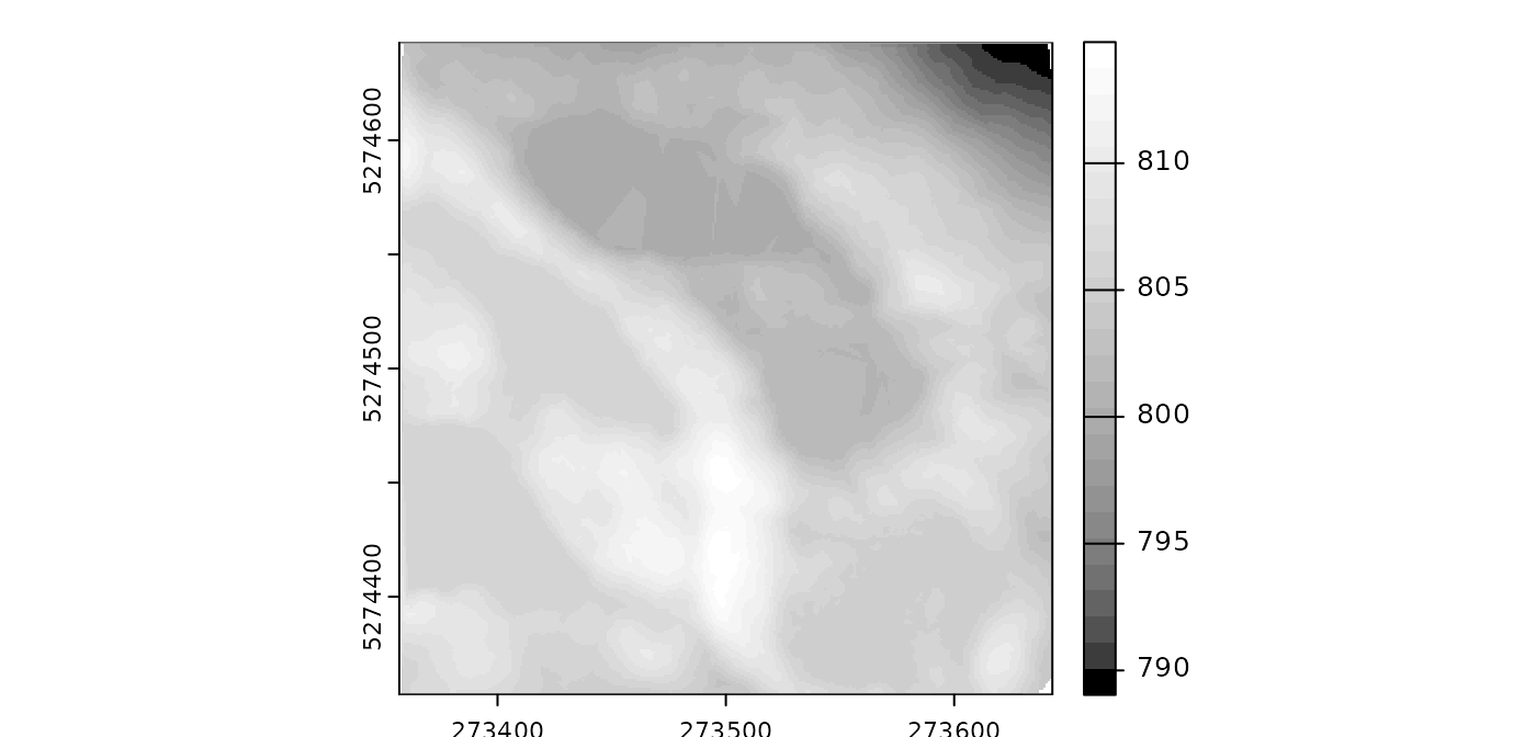

Notice that, contrary to the lidR package, there is usually no high-level function with names like rasterize_terrain(). Instead, lasR is made up of low-level functions that are more versatile but also more challenging to use.

Rasterize - internal metrics

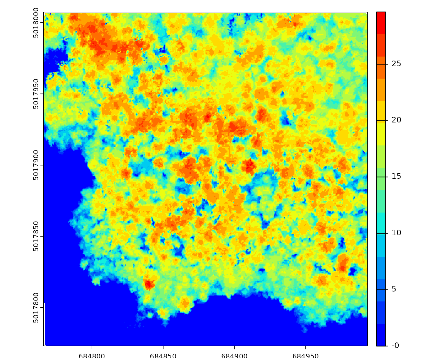
Let’s build two CHMs: one based on the highest point per pixel with a resolution of 2 meters, and the second based on the triangulation of the first returns with a resolution of 50 cm.

In the following pipeline, we are using two variations of rasterize(): one capable of rasterizing a triangulation and the other capable of rasterizing the point cloud with a predefined operator (here max). The output is a named list with two SpatRaster.

del <- triangulate(filter = keep_first())
chm1 <- rasterize(2, "max")
chm2 <- rasterize(0.5, del)
pipeline <- del + chm1 + chm2
ans <- exec(pipeline, on = f)

terra::plot(ans[[1]], mar = c(1, 1, 1, 3), col = col)
terra::plot(ans[[2]], mar = c(1, 1, 1, 3), col = col)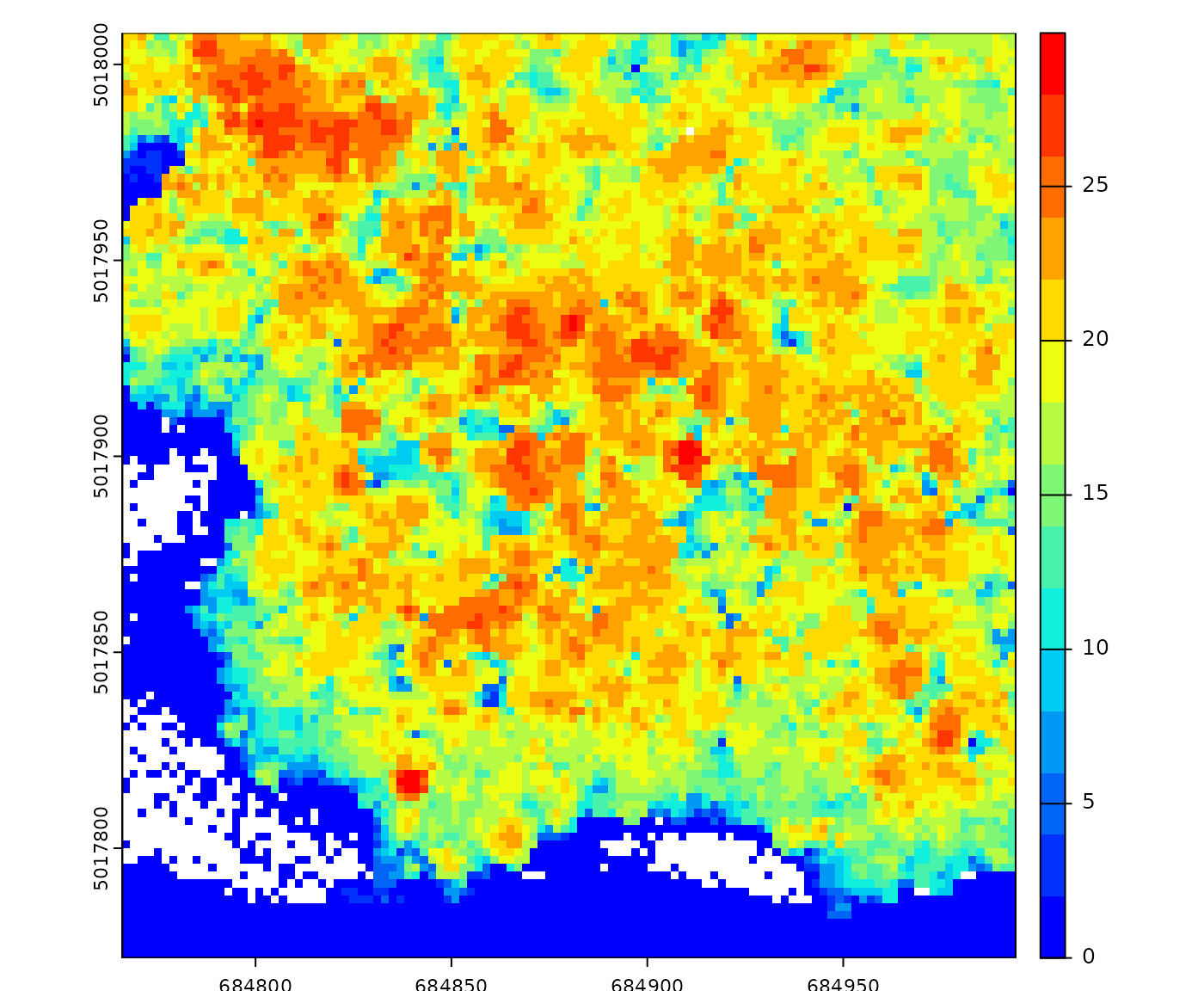

For simplicity the package has pre-installed pipelines named chm() and dtm() that do what is explained above.

Rasterize - custom metrics

Last but not least, let’s compute the map of the median intensity by injecting a user-defined expression. Like in lidR, the attributes of the point cloud are named: X, Y, Z, Intensity, gpstime, ReturnNumber, NumberOfreturns, Classification, UserData, PointSourceID, R, G, B, NIR. For users familiar with the lidR package, note that there is no ScanAngleRank/ScanAngle; instead the scanner angle is always named ScanAngle and is numeric. Also flags are named Withheld, Synthetic and Keypoint.

pipeline = rasterize(10, median(Intensity))
ans = exec(pipeline, on = f)

terra::plot(ans, mar = c(1, 1, 1, 3), col = heat.colors(15))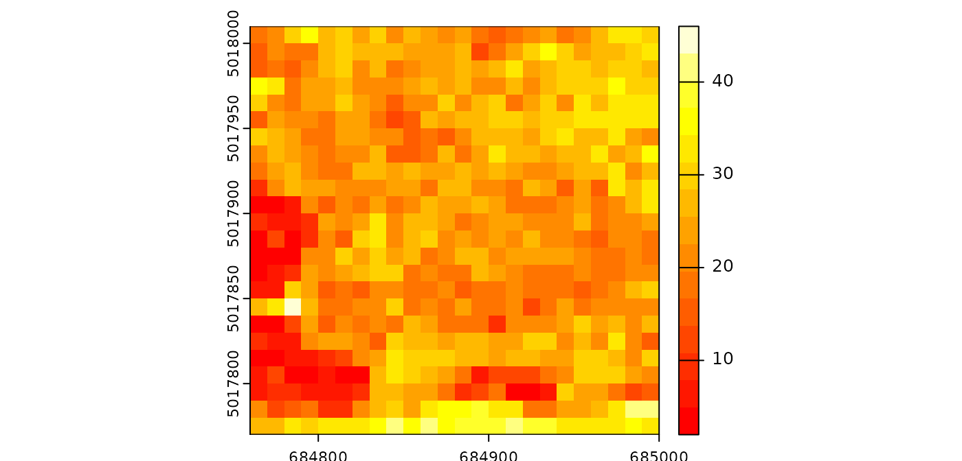

Notice that, in this specific case, using rasterize(10, "imean") is more efficient.

Rasterize - buffered

The lasR package introduced the concept of a buffered area-based approach to enhance the resolution of prediction maps. However, this concept is not covered in detail in this tutorial. For further information, readers can refer to the dedicated article

Transform with

Another way to use a Delaunay triangulation is to transform the point cloud. Users can add or subtract the triangulation from the point cloud, effectively normalizing it. Unlike the lidR package, there is no high-level function with names like normalize_points(). Instead, lasR is composed of low-level functions that offer more versatility.

Let’s normalize the point cloud using a triangulation of the ground points (meshed DTM).

In the following example, the triangulation is used by transform_with() that modifies the point cloud in the pipeline. Both triangulate() and transform_with() return nothing. The output is NULL.

del = triangulate(filter = keep_ground())
norm = transform_with(del, "-")
pipeline = del + norm
ans = exec(pipeline, on = f)
ans
#> NULL

For convenience this pipeline is pre-recorded in the package under the name normalize().

transform_with() can also transform with a raster. This is not presented in this tutorial.

To obtain a meaningful output, it is necessary to chain another stage. Here the point cloud has been modified but then, it is discarded because we did nothing with it. For instance, we can compute a Canopy Height Model (CHM) on the normalized point cloud. In the following pipeline, the first rasterization (chm1) is applied before normalization, while the second rasterization occurs after transform_with(), thus being applied to the transformed point cloud.

del = triangulate(filter = keep_ground())
norm = transform_with(del, "-")
chm1 = rasterize(2, "max")
chm2 = rasterize(2, "max")
pipeline = chm1 + del + norm + chm2
ans = exec(pipeline, on = f)

col = grDevices::colorRampPalette(c("blue", "cyan2", "yellow", "red"))(15)
terra::plot(c(ans[[1]], ans[[2]]), col = col)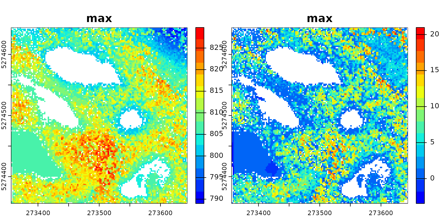

After performing normalization, users may want to write the normalized point cloud to disk for later use. In this case, you can append the write_las() stage to the pipeline.

Write LAS

write_las() can be called at any point in the pipeline. It writes one file per input file, using the name of the input files with added prefixes and suffixes. In the following pipeline, we read the files, write only the ground points to files named after the original files with the suffix _ground, perform a triangulation on the entire point cloud, followed by normalization. Finally, we write the normalized point cloud with the suffix _normalized.

write1 = write_las(paste0(tempdir(), "/*_ground.laz"), filter = keep_ground())
write2 = write_las(paste0(tempdir(), "/*_normalized.laz"), )
del = triangulate(filter = keep_ground())
norm = transform_with(del, "-")
pipeline =  write1 + del + norm + write2
ans = exec(pipeline, on = f)
ans
#>  - write_las : /tmp/Rtmptz3hfz/bcts_1_ground.laz /tmp/Rtmptz3hfz/bcts_2_ground.laz 
#>  - write_las : /tmp/Rtmptz3hfz/bcts_1_normalized.laz /tmp/Rtmptz3hfz/bcts_2_normalized.laz

It is crucial to include a wildcard * in the file path; otherwise, a single large file will be created. This behavior may be intentional. Let’s consider creating a file merge pipeline. In the following example, no wildcard * is used for the names of the LAS/LAZ files. The input files are read, and points are sequentially written to the single file dataset_merged.laz, naturally forming a merge pipeline.

ofile = paste0(tempdir(), "/dataset_merged.laz")
merge = reader_las() + write_las(ofile)
ans = exec(merge, on = f)
ans
#> [1] "/tmp/Rtmptz3hfz/dataset_merged.laz"

Callback

The callback stage holds significant importance as the second and last entry point to inject R code into the pipeline, following rasterize(). For those familiar with the lidR package, the initial step often involves reading data with lidR::readLAS() to expose the point cloud as a data.frame object in R. In contrast, lasR loads the point cloud optimally in C++ without exposing it directly to R. However, with callback, it becomes possible to expose the point cloud as a data.frame for executing specific R functions.

Similar to lidR, the attributes of the point cloud in lasR are named: X, Y, Z, Intensity, gpstime, ReturnNumber, NumberOfreturns, Classification, UserData, PointSourceID, R, G, B, NIR. Notably, for users accustomed to the lidR package, the scanner angle is consistently named ScanAngle and is numeric, as opposed to ScanAngleRank/ScanAngle. Additionally, flags are named Withheld, Synthetic, and Keypoint.

Let’s delve into a simple example. For each LAS file, the callback loads the point cloud as a data.frame and invokes the meanz() function on the data.frame.

meanz = function(data){ return(mean(data$Z)) }
call = callback(meanz, expose = "xyz")
ans = exec(call, on = f)
print(ans)
#>  - 809.0835 
#>  - 13.27202

Here the output is a list with two elements because we processed two files (f is not displayed in this document). The average Z elevation are respectively 809.08 and 13.27 in each file.

Be mindful that, for a given LAS/LAZ file, the point cloud may contain more points than the original file if the file is loaded with a buffer. Further clarification on this matter will be provided later.

The callback function is versatile and can also be employed to edit the point cloud. When the user-defined function returns a data.frame with the same number of rows as the original one, the function edits the underlying C++ dataset. This enables users to perform tasks such as assigning a class to a specific point. While physically removing points is not possible, users can flag points as Withheld. In such cases, these points will not be processed in subsequent stages, they are discarded.

edit_points = function(data)
{
  data$Classification[5:7] = c(2L,2L,2L)
  data$Withheld = FALSE
  data$Withheld[12] = TRUE
  return(data)
}

call = callback(edit_points, expose = "xyzc")
ans = exec(call, on = f)
ans
#> NULL

As observed, here, this time callback does not explicitly return anything; however, it edited the point cloud internally. To generate an output, users must use another stage such as write_las(). It’s important to note that write_las() will NOT write the point number 12 which is flagged withheld. Neither any subsequent stage will process it. The point is still in memory but is discarded.

For memory and efficiency reasons, it is not possible to physically remove a point from the underlying memory in lasR. Instead, the points flagged as withheld will never be processed. One consequence of this, is that points flagged as withheld in a LAS/LAZ file will not be processed in lasR. This aligns with the intended purpose of the flag according to the LAS specification but may differ from the default behavior of many software on the market including lidR.

Now, let’s explore the capabilities of callback further. First, let’s create a lidR-like read_las() function to expose the point cloud to R. In the following example, the user-defined function is employed to return the data.frame as is. When the user’s function returns a data.frame with the same number of points as the original dataset, this updates the points at the C++ level. Here, we use no_las_update = TRUE to explicitly return the result.

read_las = function(f, select = "xyzi", filter = "")
{
  load = function(data) { return(data) }
  read = reader_las(filter = filter)
  call = callback(load, expose = select, no_las_update = TRUE)
  return (exec(read+call, on = f))
}

f <- system.file("extdata", "Topography.las", package="lasR")
las = read_las(f)
head(las)
#>          X       Y        Z Intensity
#> 1 273357.1 5274360 806.5340      1340
#> 2 273357.2 5274359 806.5635       728
#> 3 273357.2 5274358 806.0248      1369
#> 4 273357.2 5274510 809.6303       589
#> 5 273357.2 5274509 809.3880      1302
#> 6 273357.2 5274508 809.4847       123

Ground points can also be classified using an R function, such as the one provided by the RCSF package:

csf = function(data)
{
  id = RCSF::CSF(data)
  class = integer(nrow(data))
  class[id] = 2L
  data$Classification <- class
  return(data)
}

read = reader_las()
classify = callback(csf, expose = "xyz")
write = write_las()
pipeline = read + classify + write
exec(pipeline, on = f)

callback() exposes the point cloud as a data.frame. This is the only way to expose the point clouds to users in a manageable way. One of the reasons why lasR is more memory-efficient and faster than lidR is that it does not expose the point cloud as a data.frame. Thus, the pipelines using callback() are not significantly different from lidR. The advantage of using lasR here is the ability to pipe different stages.

Local maximum

This stage works either on the point cloud or a raster. In the following pipeline the first stage builds a CHM, the second stage finds the local maxima in the point cloud and the second stages finds the local maxima in the chm. lm1 and lm2 are expected to produce relatively close results but not strictly identical.

chm = rasterize(1, "max")
lm1 = local_maximum(3)
lm2 = local_maximum_raster(chm, 3)
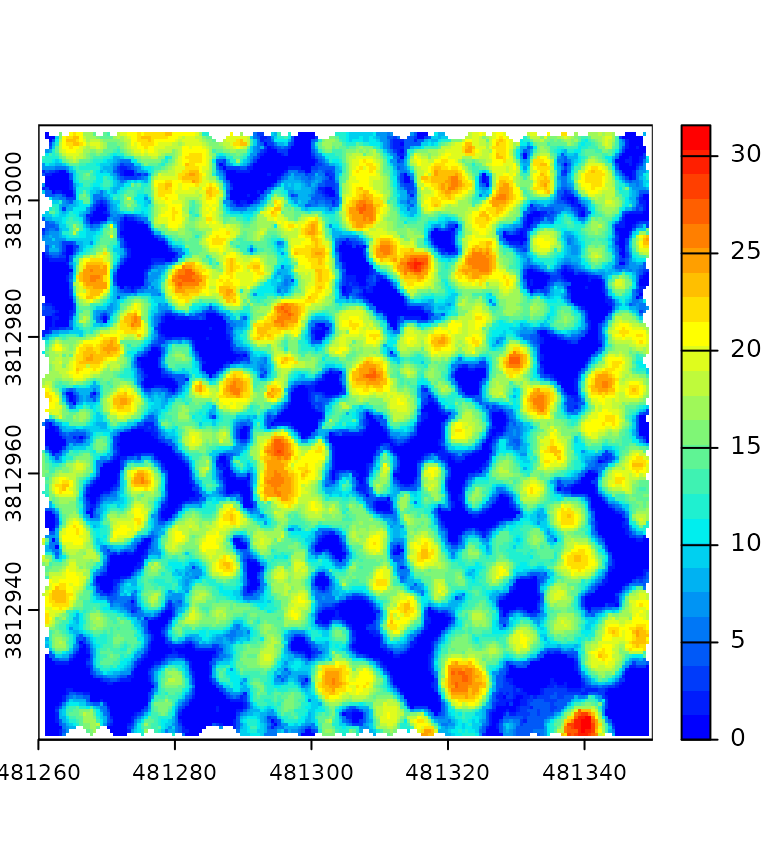
pipeline = chm + lm1 + lm2

Tree Segmentation

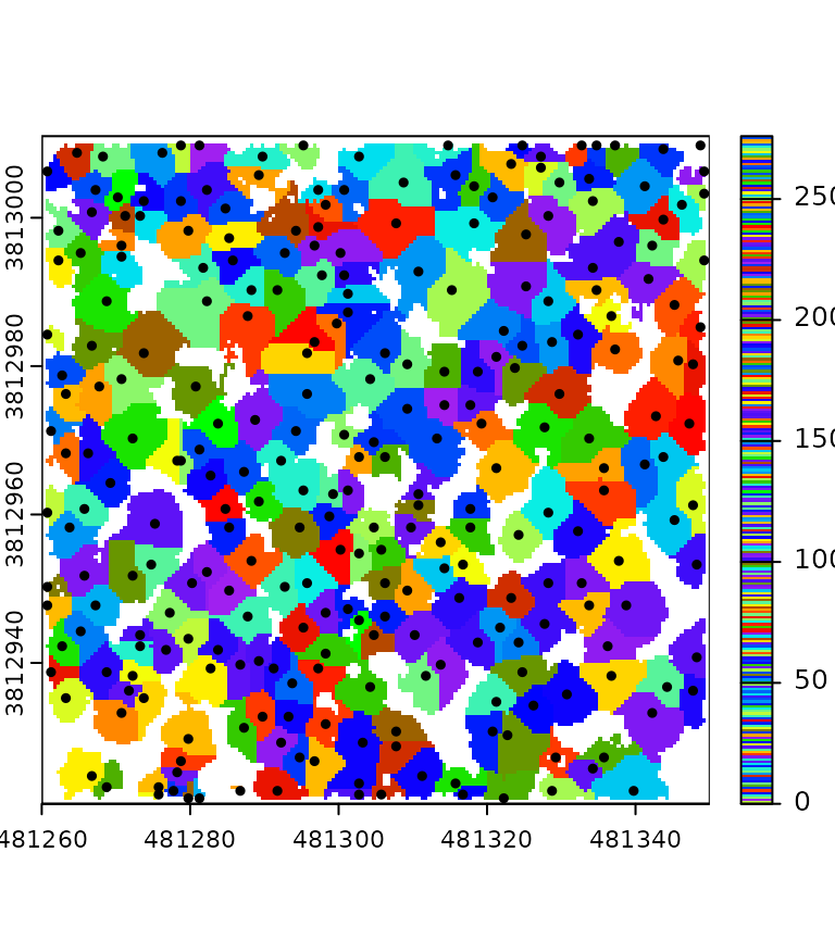
This section presents a complex pipeline for tree segmentation using local_maximum_raster() to identify tree tops on a CHM. It uses region_growing() to segment the trees using the seeds produced by local_maximum_raster(). The Canopy Height Model (CHM) is triangulation-based using triangulation() and rasterize() in the first returns. The CHM is post-processed with pit_fill(), an algorithm designed to enhance the CHM by filling pits and NAs. The reader may have noticed that the seeds are produced with the same raster than the one used in region_growing(). This is checked internally to ensure the seeds are matching the raster used for segmenting the trees.

In this tutorial, the pipeline is tested on one file to render the page faster. However, this pipeline can be applied to any number of files and will produce a continuous output, managing the buffer between files. Every intermediate output can be exported, and in this tutorial, we export everything to display all the outputs.

del = triangulate(filter = keep_first())
chm = rasterize(0.5, del)
chm2 = pit_fill(chm)
seed = local_maximum_raster(chm2, 3)
tree = region_growing(chm2, seed)
pipeline = del + chm + chm2 +  seed + tree
ans = exec(pipeline, on = f)

col = grDevices::colorRampPalette(c("blue", "cyan2", "yellow", "red"))(25)
col2 = grDevices::colorRampPalette(c("purple", "blue", "cyan2", "yellow", "red", "green"))(50)
terra::plot(ans$rasterize, col = col, mar = c(1, 1, 1, 3))
terra::plot(ans$pit_fill, col = col, mar = c(1, 1, 1, 3))
terra::plot(ans$region_growing, col = col2[sample.int(50, 277, TRUE)], mar = c(1, 1, 1, 3))
plot(ans$local_maximum$geom, add = T, pch = 19, cex = 0.5)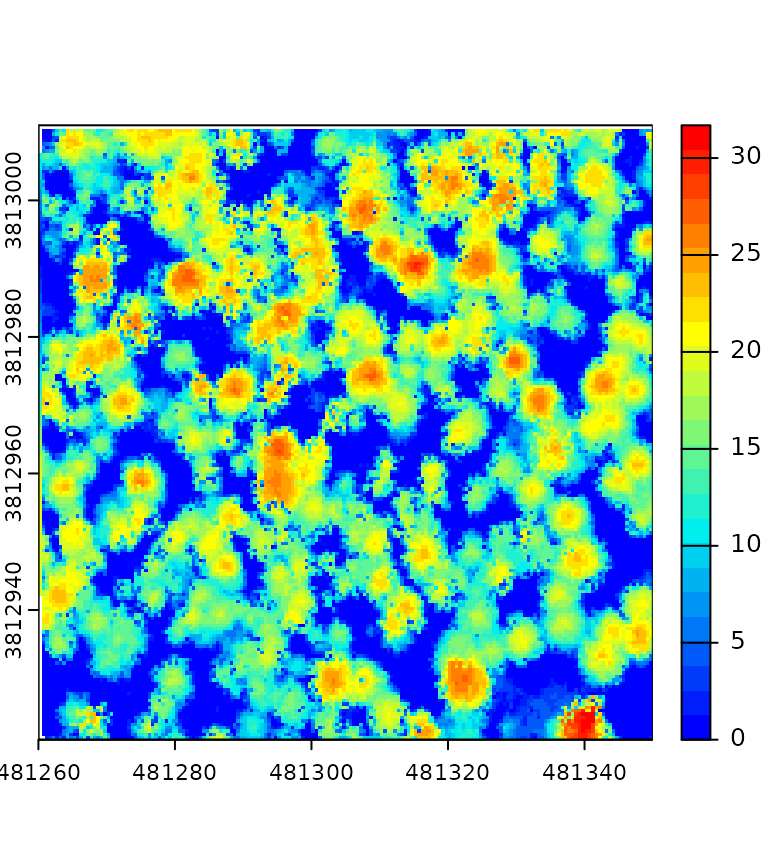

Buffer

Point clouds are typically stored in multiple contiguous files. To avoid edge artifacts, each file must be loaded with extra points coming from neighboring files. Everything is handled automatically, except for the callback() stage. In callback(), the point cloud is exposed as a data.frame with the buffer, providing the user-defined function with some spatial context. If callback is used to edit the points, everything is handled internally. However, if an R object is returned, it is the responsibility of the user to handle the buffer.

For example, in the following pipeline, we are processing two files, and callback() is used to count the number of points. The presence of triangulate() implies that each file will be loaded with a buffer to make a valid triangulation. Consequently, counting the points in callback() returns more points than summarise() because summarise() is an internal function that knows how to deal with the buffer.

count = function(data) { length(data$X) }
del = triangulate(filter = keep_ground())
npts = callback(count, expose = "x")
sum = summarise()
ans = exec(del + npts + sum, on = f)
print(ans$callback)
#>  - 682031 
#>  - 931581
ans$callback[[1]]+ ans$callback[[2]]
#> [1] 1613612
ans$summary$npoints
#> [1] 1355607

We can compare this with the pipeline without triangulate(). In this case, there is no reason to use a buffer, and the files are not buffered. The counts are equal.

ans = exec(npts + sum, on = f)
ans$callback[[1]]+ ans$callback[[2]]
#> [1] 1355607
ans$summary$npoints
#> [1] 1355607

To handle the buffer, the user can read the attribute bbox of the data.frame. It contains the bounding box of the point cloud without the buffer or use the column Buffer that contains TRUE or FALSE for each point. If TRUE, the point is in the buffer. The buffer is exposed only if the user includes the letter 'b'.

count_buffer_aware = function(data) {
  bbox = attr(data, "bbox")
  npoints = sum(!data$Buffer)
  return(list(bbox = bbox, npoints = npoints))
}

del = triangulate(filter = keep_ground())
npts = callback(count_buffer_aware, expose = "b") # b for buffer
sum = summarise()
ans = exec(del + npts + sum, on = f)
print(ans$callback)
#>  - List:
#>    - bbox : 885022.4 629157.2 885210.2 629400 
#>    - npoints : 531662 
#>  - List:
#>    - bbox : 885024.1 629400 885217.1 629700 
#>    - npoints : 823945
ans$callback[[1]]$npoints+ ans$callback[[2]]$npoints
#> [1] 1355607
ans$summary$npoints
#> [1] 1355607

In conclusion, in the hypothesis that the user-defined function returns something complex, there are two ways to handle the buffer: either using the bounding box or using the Buffer flag. A third option is to use drop_buffer. In this case users ensure to receive a data.frame that does not include points from the buffer.

Hulls

A Delaunay triangulation defines a convex polygon, which represents the convex hull of the points. However, in dense point clouds, removing triangles with large edges due to the absence of points results in a more complex structure.

del = triangulate(15, filter = keep_ground(), ofile = tempgpkg())
ans = exec(del, on = f)

par(mar = c(2, 2, 1, 1))
plot(ans, axes = T, lwd = 0.5)

The hulls() algorithm computes the contour of the mesh, producing a concave hull with holes:

del = triangulate(15, filter = keep_ground())
bound = hulls(del)
ans = exec(del+bound, on = f)

par(mar = c(2, 2, 1, 1))
plot(ans, axes = T, lwd = 0.5, col = "gray")

However hulls() is more likely to be used without a triangulation. In this case it returns the bounding box of each LAS/LAZ file read from the header. And if it is used with triangulate(0) it returns the convex hull but this is a very inefficient way to get the convex hull.

Sampling Voxel

The sampling_voxel() and summarise() functions operate similarly to other algorithms, and their output depends on their position in the pipeline:

pipeline = summarise() + sampling_voxel(4) + summarise()
ans = exec(pipeline, on = f)
print(head(ans[[1]]))
#>  - npoints : 73403 
#>  - nsingle : 31294 
#>  - nwithheld : 0 
#>  - nsynthetic : 0 
#>  - npoints_per_return : 53538 15828 3569 451 16 1 
#>  - npoints_per_class : 61347 8159 3897
print(head(ans[[2]]))
#>  - npoints : 12745 
#>  - nsingle : 5117 
#>  - nwithheld : 0 
#>  - nsynthetic : 0 
#>  - npoints_per_return : 9436 2600 616 90 3 
#>  - npoints_per_class : 10809 1571 365

Readers

reader_las() MUST be the first stage of each pipeline even if it can conveniently be omitted in its simplest form. However there are several readers hidden behind reader_las():

reader_las_coverage(): will read of the files and process the entire point cloud. This is the default behavior of reader_las().
reader_las_rectangles(): will read only some rectangular regions of interest of the coverage and process then sequentially.
reader_las_circles(): will read only some circular regions of interest of the coverage and process then sequentially.

The following pipeline triangulates the ground points, normalizes the point cloud, and computes some metric of interest for each file of the entire coverage. Each file is loaded with a buffer so that triangulation is performed without edge artifacts. Notice the use of drop_buffer = TRUE to expose the data.frame without the buffer used to perform the triangulation and normalization.

my_metric_fun = function(data) { mean(data$Z) }
tri <- triangulate(filter = keep_ground())
trans <- transform_with(tri)
norm <- tri + trans
metric <- callback(my_metric_fun, expose = "z", drop_buffer = TRUE)
pipeline = norm + metric

The following pipeline, on the contrary, works exactly the same but operates only on circular plots.

pipeline = reader_las_circles(xcenter, ycenter, 11.28) + pipeline

These readers allow building a ground inventory pipeline, or a plot extraction for examples

Plot inventory

This pipeline extracts a plot inventory using a shapefile from a non-normalized point cloud, normalizes each plot, computes metrics for each plot, and writes each normalized and non-normalized plot in separate files. Each circular plot is loaded with a buffer to perform a correct triangulation. The plots are exposed to R without the buffer using drop_buffer = TRUE.

ofiles_plot <- paste0(tempdir(), "/plot_*.las")
ofiles_plot_norm <- paste0(tempdir(), "/plot_*_norm.las")

my_metric_fun = function(data) { mean(data$Z) }

library(sf)
inventory <- st_read("shapefile.shp")
coordinates <- st_coordinates(inventory)
xcenter <- coordinates[,1]
ycenter <- coordinates[,2]

read <- reader_las(xc = xcenter, yc = ycenter, r = 11.28) 
tri <- triangulate(filter = keep_ground())
trans <- transform_with(tri)
norm <- tri + trans
metric <- callback(my_metric_fun, expose = "z", drop_buffer = TRUE)
write1 <- write_las(ofiles_plot)
write2 <- write_las(ofiles_plot_norm)

pipeline = read + trans + write1 + norm + write2

Wildcard Usage

Usually, write_las() is used with a wildcard in the ofile argument (see above) to write one file per processed file. Otherwise, everything is written into a single massive LAS file (which might be the desired behavior). On the contrary, rasterize() is used without a wildcard to write everything into a single raster file, but it also accepts a wildcard to write the results in multiple files, which is very useful with reader_las_circles() to avoid having one massive raster mostly empty. Compare this pipeline with and without the wildcard.

Without a wildcard, the output is a single raster that covers the entire point cloud with two patches of populated pixels.

ofile = paste0(tempdir(), "/chm.tif")   # no wildcard

x = c(885100, 885100)
y = c(629200, 629600)

pipeline = reader_las(xc = x, yc = y, r = 20) + rasterize(2, "max", ofile = ofile)
r0 = exec(pipeline, on = f)

terra::plot(r0, col = col) # covers the entire collection of files

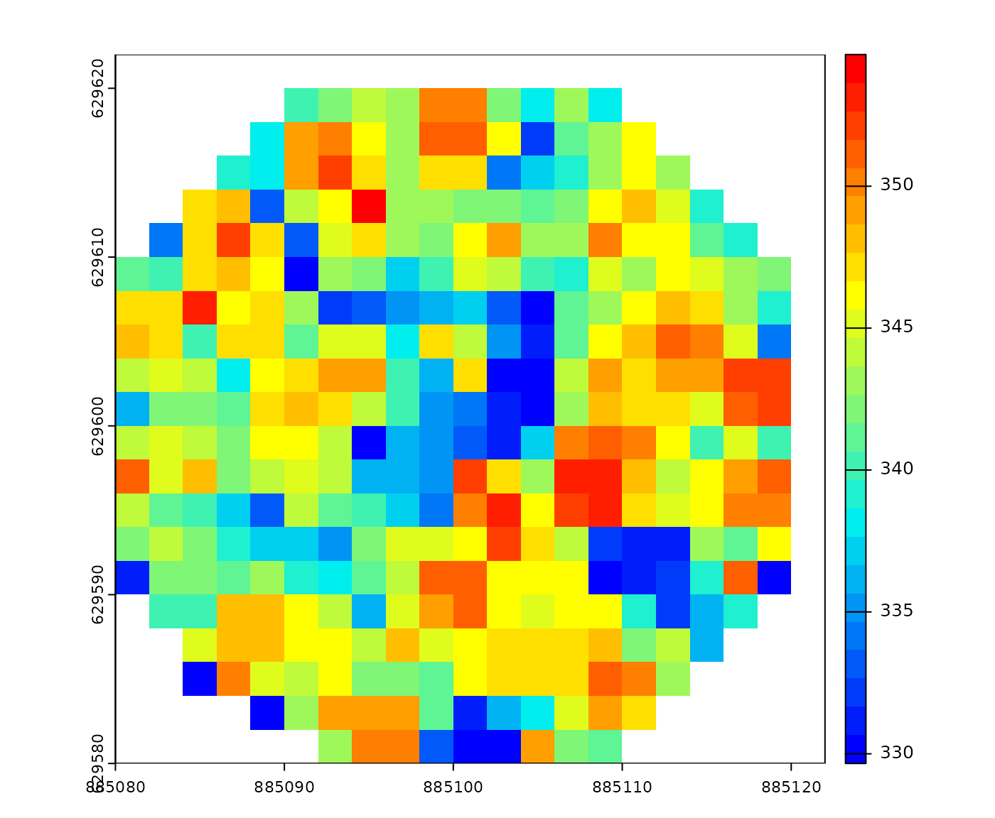
With a wildcard, the output contains two rasters that cover regions of interest.

ofile = paste0(tempdir(), "/chm_*.tif") # wildcard

x = c(885100, 885100)
y = c(629200, 629600)

pipeline = reader_las(xc = x, yc = y, r = 20) + rasterize(2, "max", ofile = ofile)
ans = exec(pipeline, on = f)

r1 = terra::rast(ans[1])
r2 = terra::rast(ans[2])
terra::plot(r1, col = col)
terra::plot(r2, col = col)

Compatibility with lidR

While lasR does not depends on lidR it has some compatibility with it. Instead of providing paths to files or folder it is possible to pass a LAScatalog or a LAS object to the readers.

library(lasR)
library(lidR)

pipeline = normalize() + write_las()

ctg = readLAScatalog(folder)
ans = exec(pipeline, on = ctg)

las = readLAS(file)
ans = exec(pipeline, on = las)

In the case of a LAScatalog, exec() respects the processing options of the LAScatalog including the chunk size, chunk buffer, progress bar display and partial processing. In the general case, the same options can be supplied as arguments of the exec() functions.

Parallel processing

The topic is covered in a dedicated article

Jean-Romain Roussel