13  Derived metrics at the voxel level

13.1 Overview

The “voxel” level of regularization corresponds to the computation of derived metrics for regularly spaced location in 3D. The voxel_metrics() function allows calculation of voxel-based metrics on provided point clouds and works like cloud_metrics(), grid_metrics(), and tree_metrics() seen in Chapter 9, Chapter 10, Chapter 11 and Chapter 12. In the examples below we use the Megaplot.laz data set, but the potential to use voxel_metrics() is particularly interesting for dense point clouds such as those produced by terrestrial lidar, or digital photogrammetry.

13.2 Applications

We can count the number of points inside each 4 x 4 x 4 m voxel:

LASfile <- system.file("extdata", "Megaplot.laz", package="lidR")
las <- readLAS(LASfile) # read file
vox_met <- voxel_metrics(las, ~list(N = length(Z)), 4) # calculate voxel metrics

In this example the point cloud is first converted into 4 m voxels, then the function length(Z) is applied to all points located inside every voxel. The output is a data.table that contains the X, Y, and Z coordinates of voxels, and the calculated number of points and can be visualized in 3D using the plot() function as follows:

plot(vox_met, color="N", pal = heat.colors, size = 4, bg = "white", voxel = TRUE)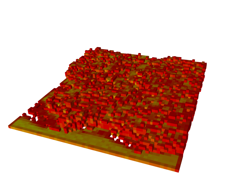

Similarly to other *_metrics() functions designed to calculate derived metrics, voxel_metrics() can be used to calculate any number of pre- or user-defined summaries. For example, to calculate minimum, mean, maximum, and standard deviation of intensity in each voxel we can create a following function:

custom_metrics <- function(x) { # user-defined function
  m <- list(
    i_min = min(x),
    i_mean = mean(x),
    i_max = max(x),
    i_sd = sd(x)
  )
  return(m) # output
}

vox_met <- voxel_metrics(las, ~custom_metrics(Intensity), 4) # calculate voxel metrics