6  Instance Segmentation

Instance segmentation is the process of assigning a label to individual objects within a dataset. In our case, the objective is to assign a unique ID to each tree.

The entire pipeline can be summarized in just two lines of code.

seeds <- find_seeds(las, params)
las   <- segment_instance(las, seeds, params)

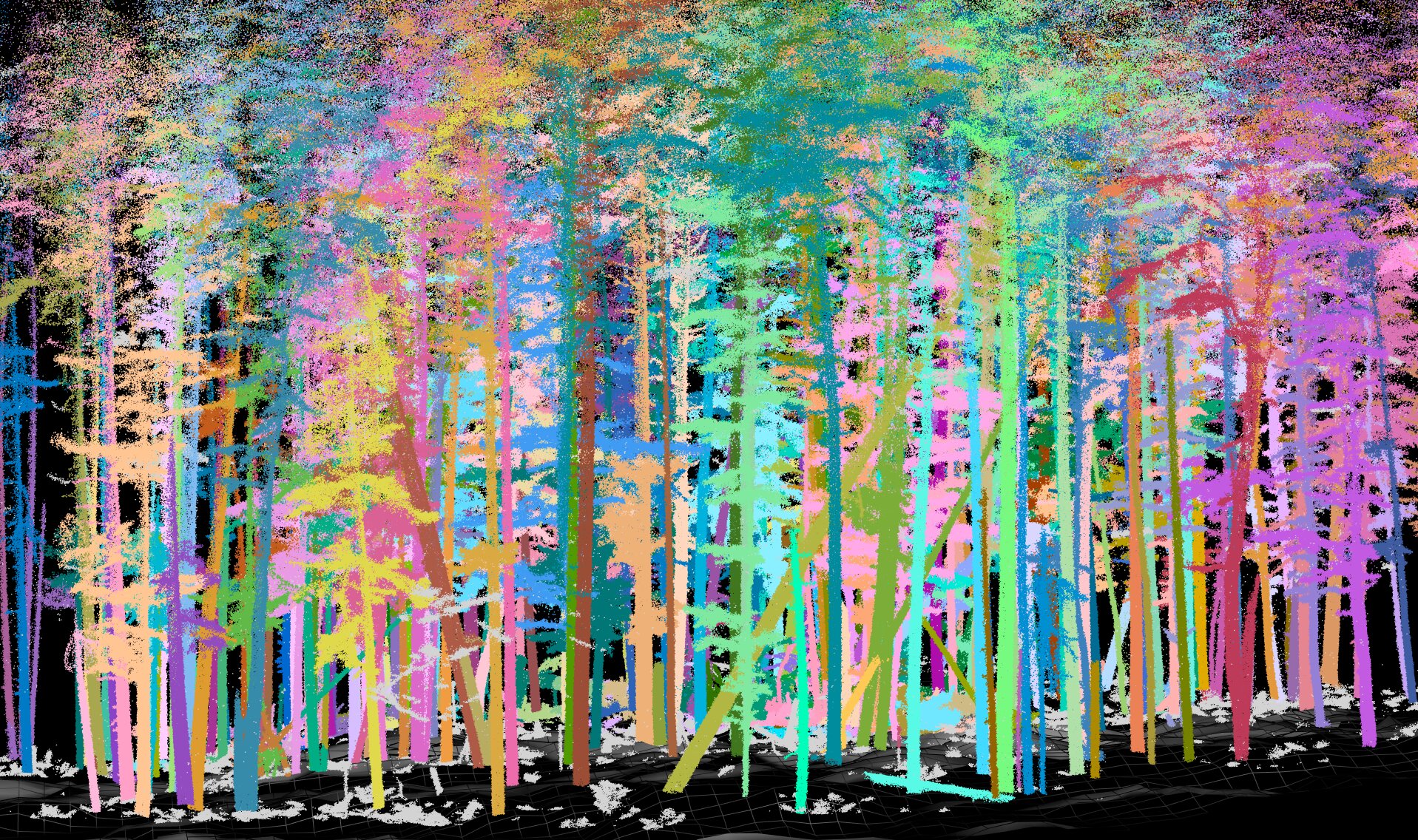
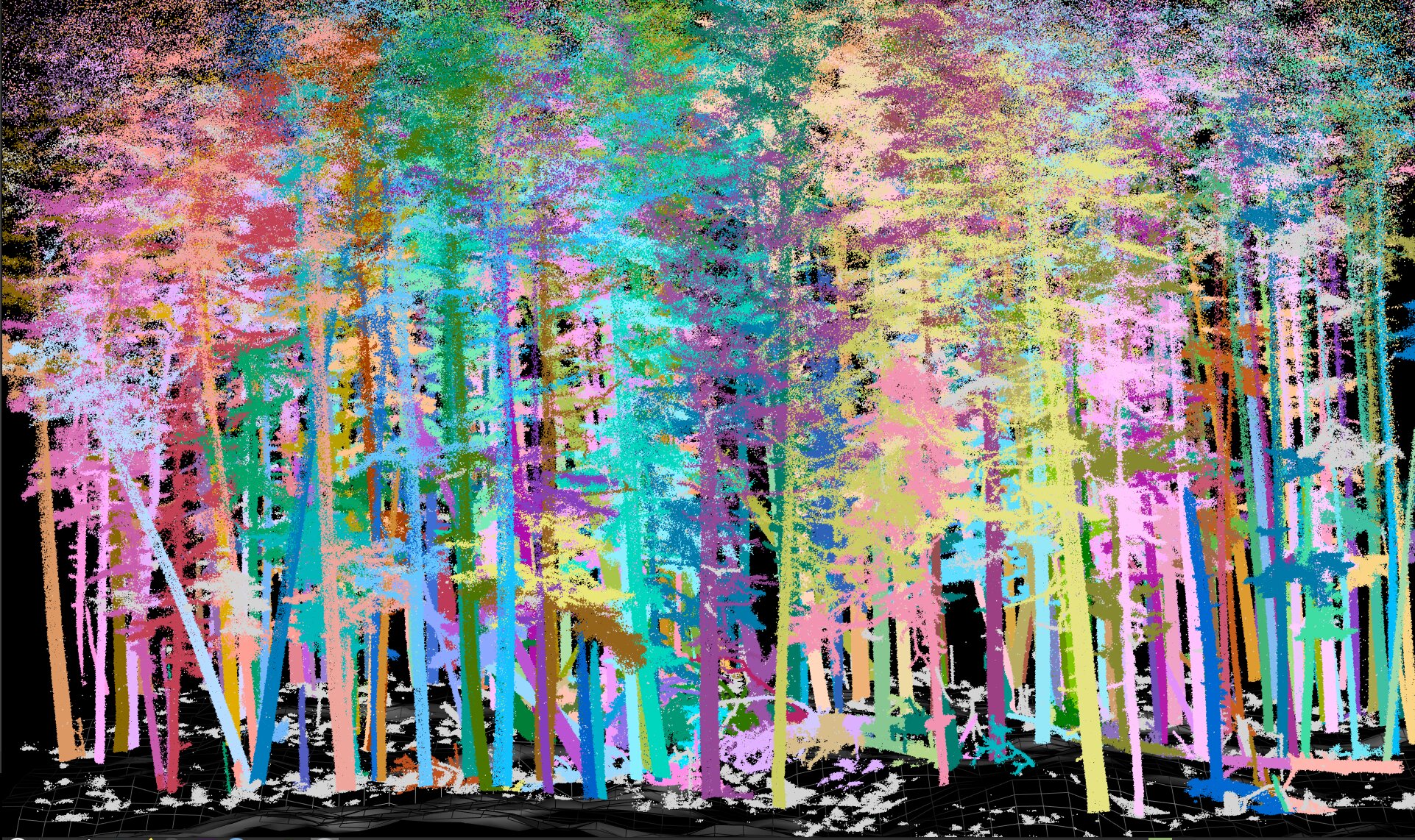
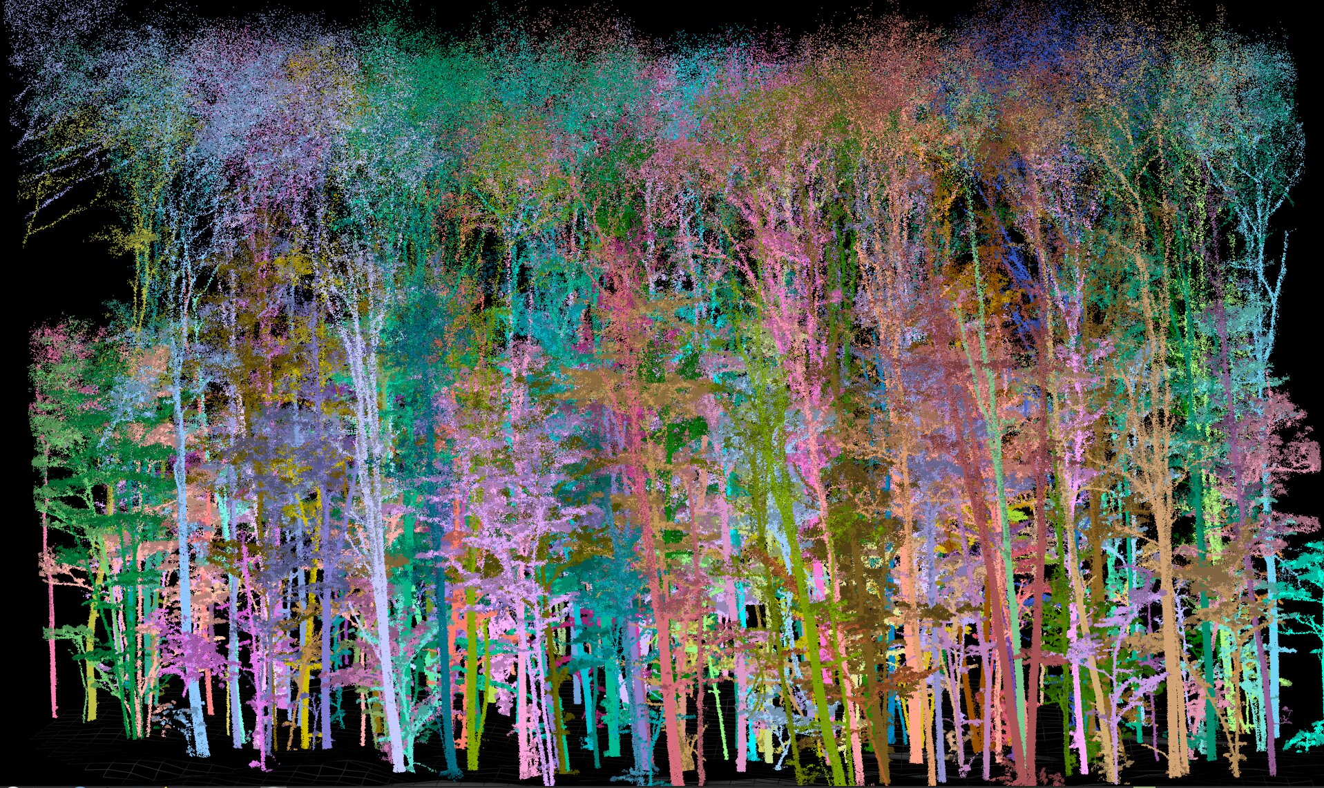
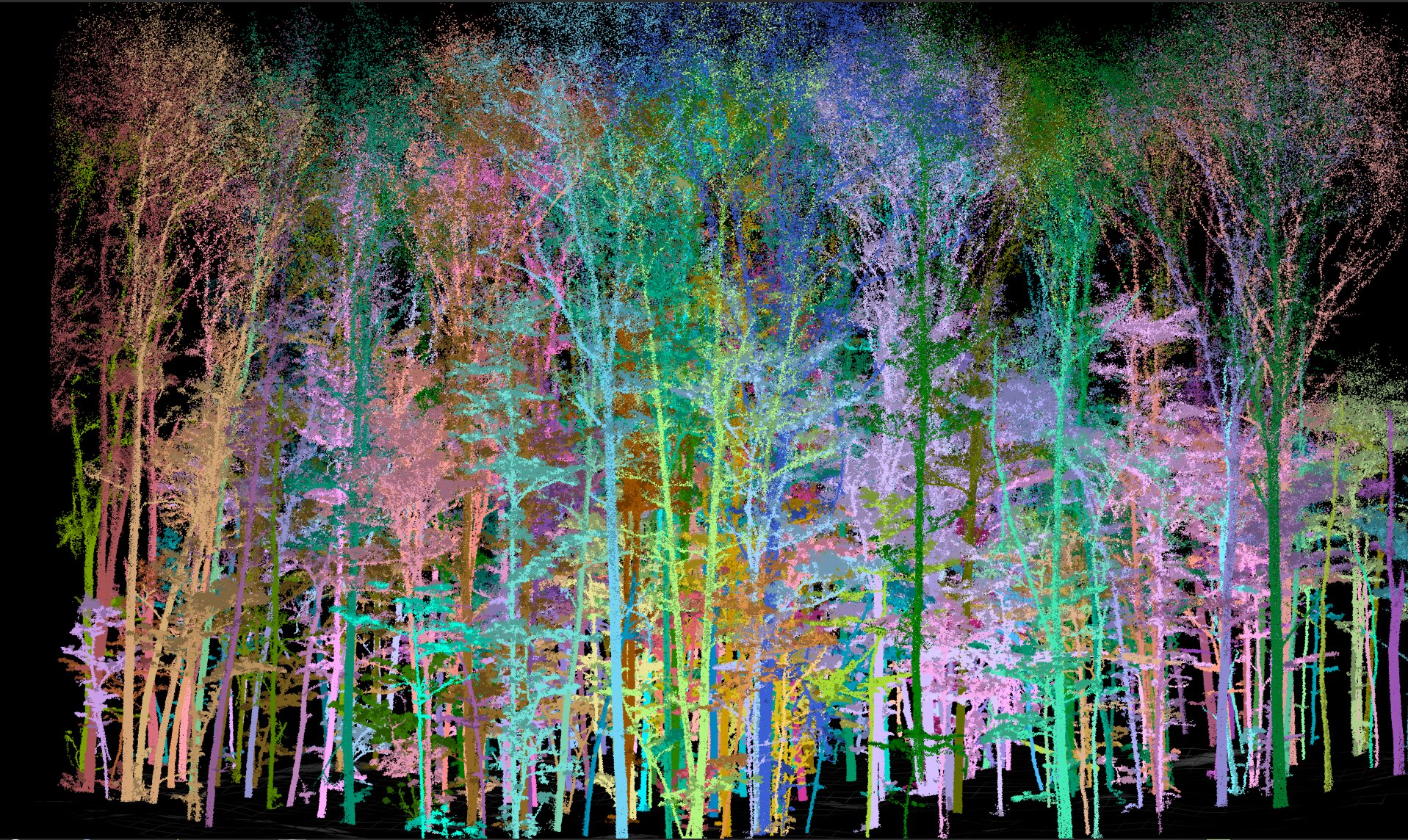
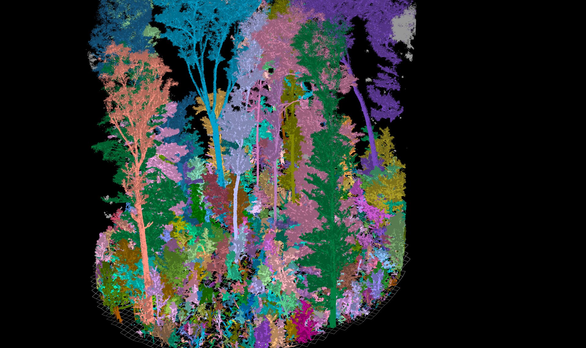
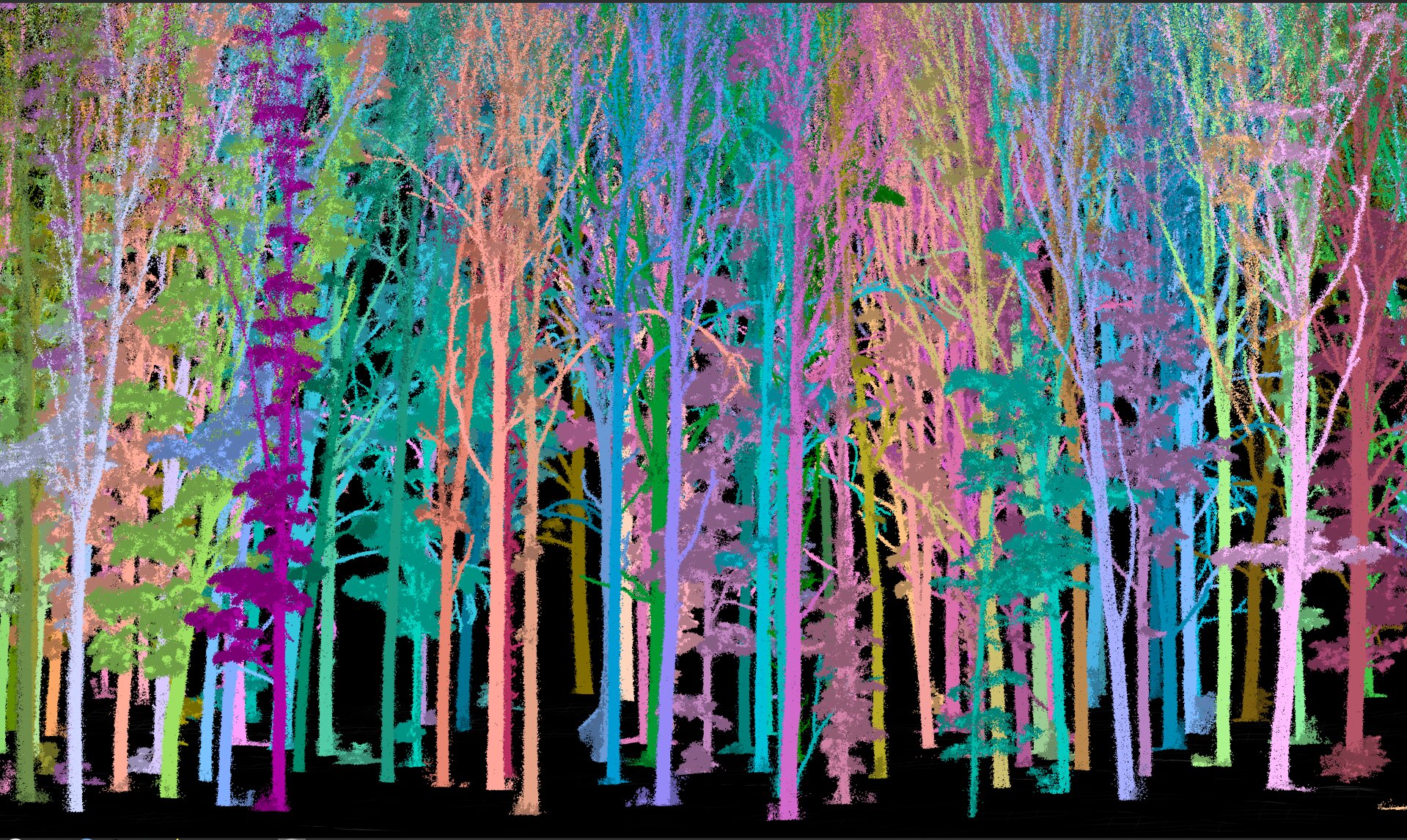
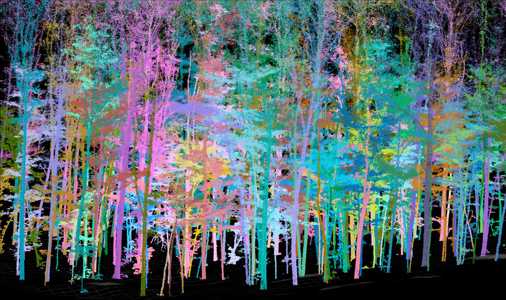
Below a gallery of semantic segmentation for various datasets

6.1 Seeds

seeds = find_seeds(las, params)

In order to segment each tree individually, we first need to locate every tree. This step is the most critical, sensitive, and improvable stage of the entire pipeline. Detecting every tree, sapling, and bush accurately, without a single error, is highly challenging, especially in complex contexts, but it is essential for proper semantic segmentation.

Segmenting individual bushes, for example, is necessary to isolate them and ensure they are not mistakenly assigned to a nearby tree.

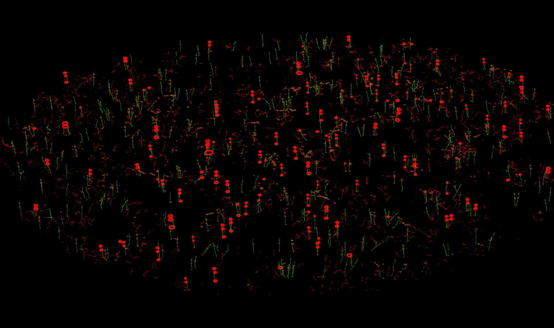
The method relies on the pathfinder used in the semantic segmentation process described in the previous chapter. As we saw before, we were tracking passage points to reach the ground. The current pipeline uses these passage points along with the wood/foliage semantic segmentation to isolate each tree, sapling, or bush.

In the previous stage of semantic segmentation we ended up with passage points after using a pathfinder

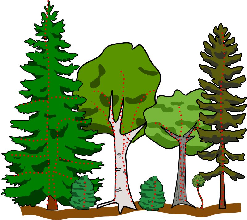
It is possible to have multiple passages for a given tree. The pathfinder cannot pass through the centerline of the trunk because there are no points there. Instead, it follows the shortest path, and depending on the starting points, multiple paths may be created. Typically, there are three or four hotspots per big tree and many more for massive tropical trees.

Simple view of passage points

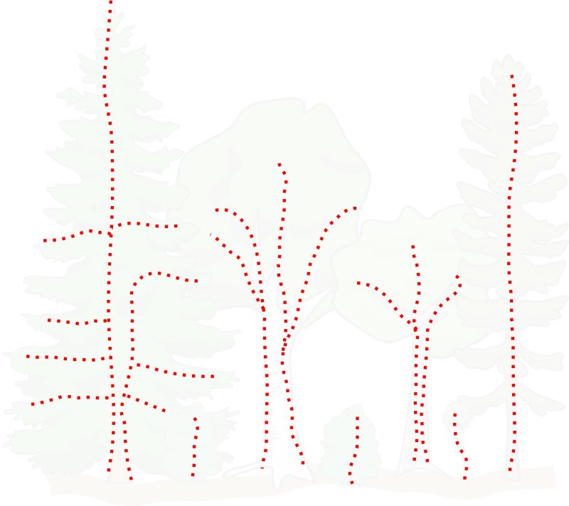
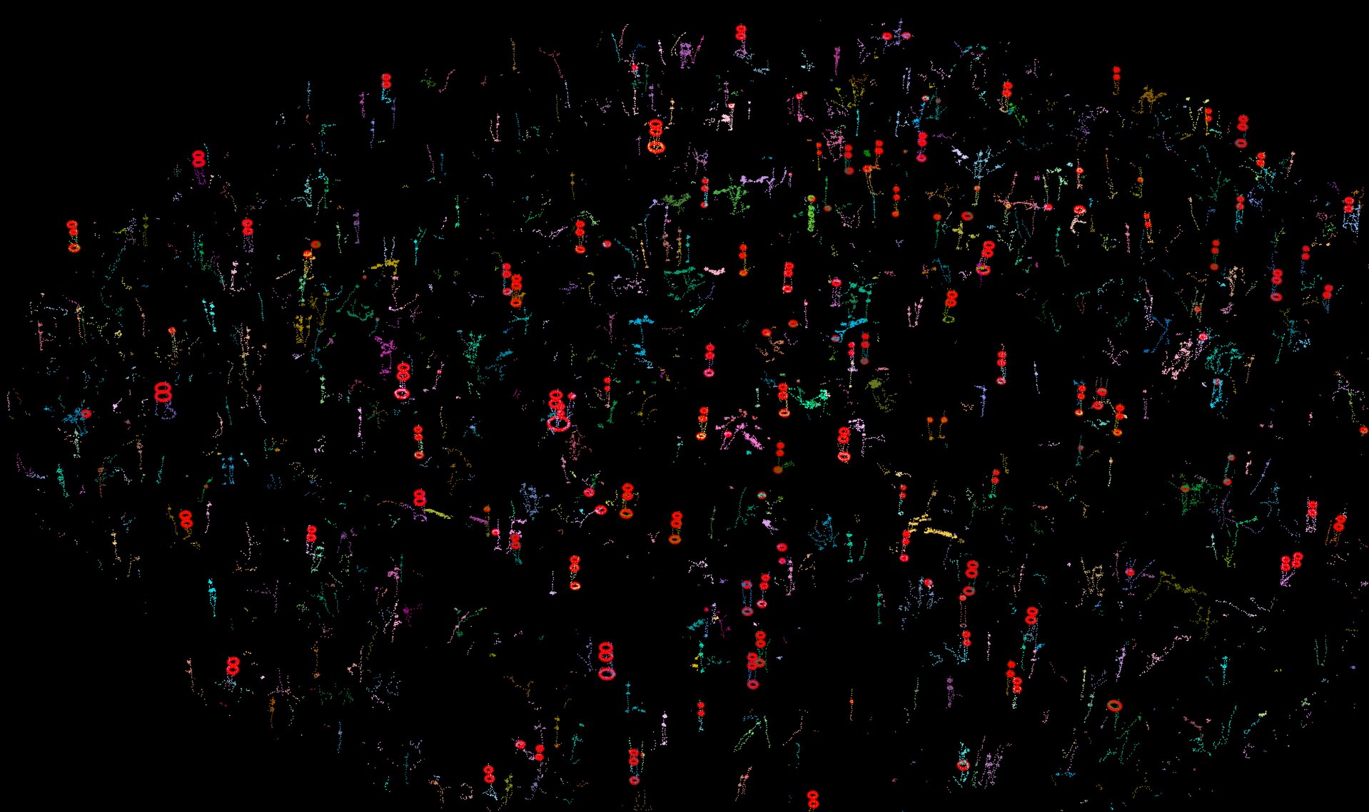
These passage points are connected and assigned an ID. However, since a tree can often have two or more passage paths, it may end up with multiple IDs.

After connecting the passage points we often have several IDs per tree

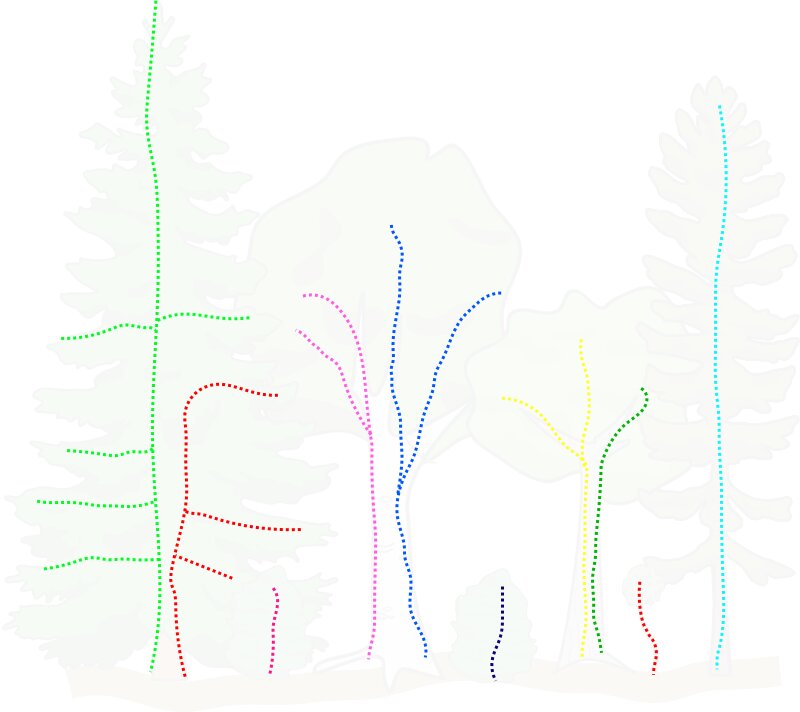
To merge the different paths for each tree, we use the semantic segmentation. The paths are expected to be connected by wood, and since we have wood classification, we can extract wood points from the lower layers and apply a connected component analysis. This merges paths that are physically connected by wood.

Several paths per individual trees are connected by wood points

Individual paths are merged through wood points into coherent tree identification

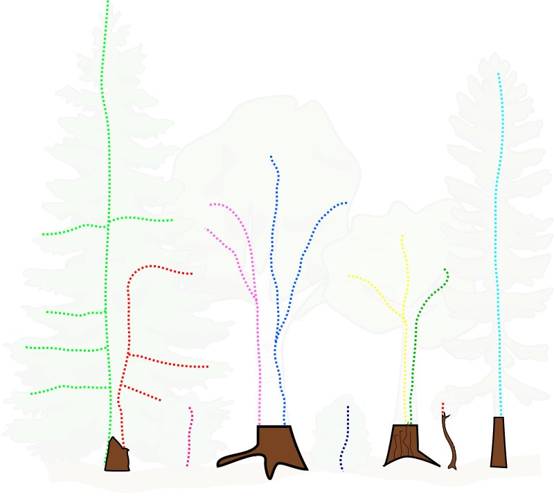
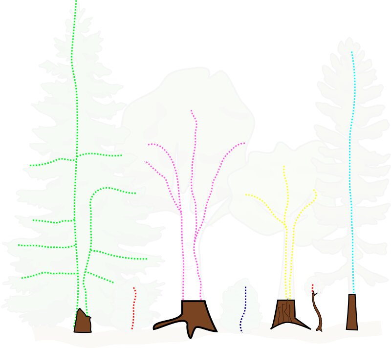
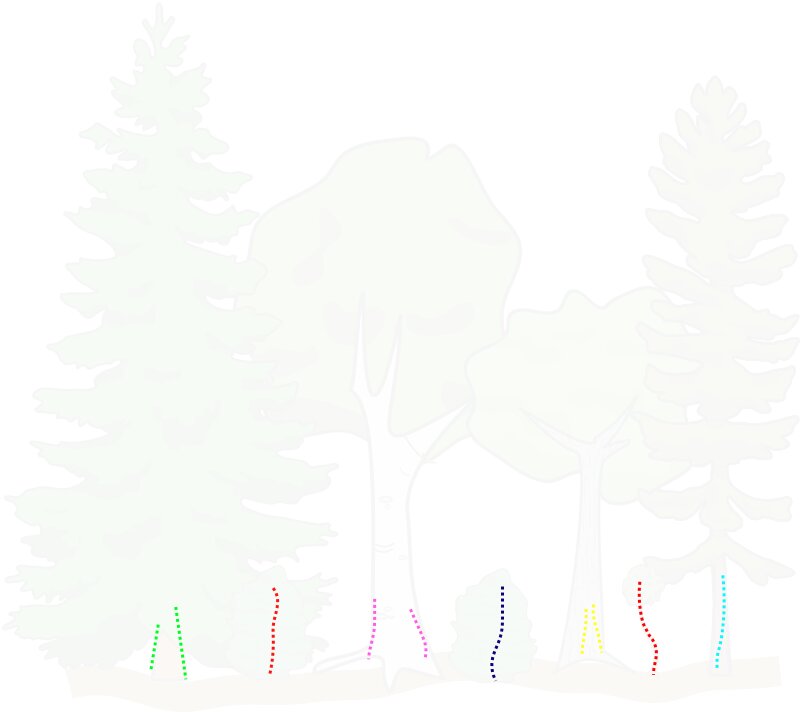
Finally, we keep only the passage points that are close to the ground to avoid complications in more complex forest contexts.

While the previous sketches may make the process seem straightforward, in practice, passage points are often interleaved among branches. False positives and false negatives in wood points can occur. Real scenes are far more complex than these sketches, requiring careful analysis and additional constraints. Nevertheless, the sketches convey the main idea, despite the full algorithm being more intricate. An example of a real scene is shown in the next sections.

Final seeds used to assign an ID to each tree

6.2 Pathfinder

las <- segment_instance(las, seeds, params)

To assign an ID to each tree, the pipeline uses a pathfinder to locate the closest seed. We won’t dive deeply into the pathfinder here, but four key principles are essential to remember:

1. Shortest path: For each point, we search for the shortest path to a seed and retain the tree ID of that seed.
   
2. Cost function: The path cost is based on the cube of the distance between neighboring points, which favors traversal through dense areas and avoids low-density gaps.
   
3. Angle penalty: The cost is penalized based on the angle between points, encouraging vertical, downward paths.
   
4. Semantic penalty: The cost is penalized according to the wood/foliage segmentation. Moving from wood to foliage is extremely expensive; moving from foliage to foliage incurs a significant extra cost. Moving from foliage to wood is favored, while moving from wood to wood has the regular cost.

These mechanisms ensure that the pathfinder primarily travels through wood and almost never moves from wood to foliage, protecting against incorrect tree ID assignments.

Final segmentation. Each point of the point cloud is assigned the ID of the closest seed using a pathfinder

6.3 Real Rendering

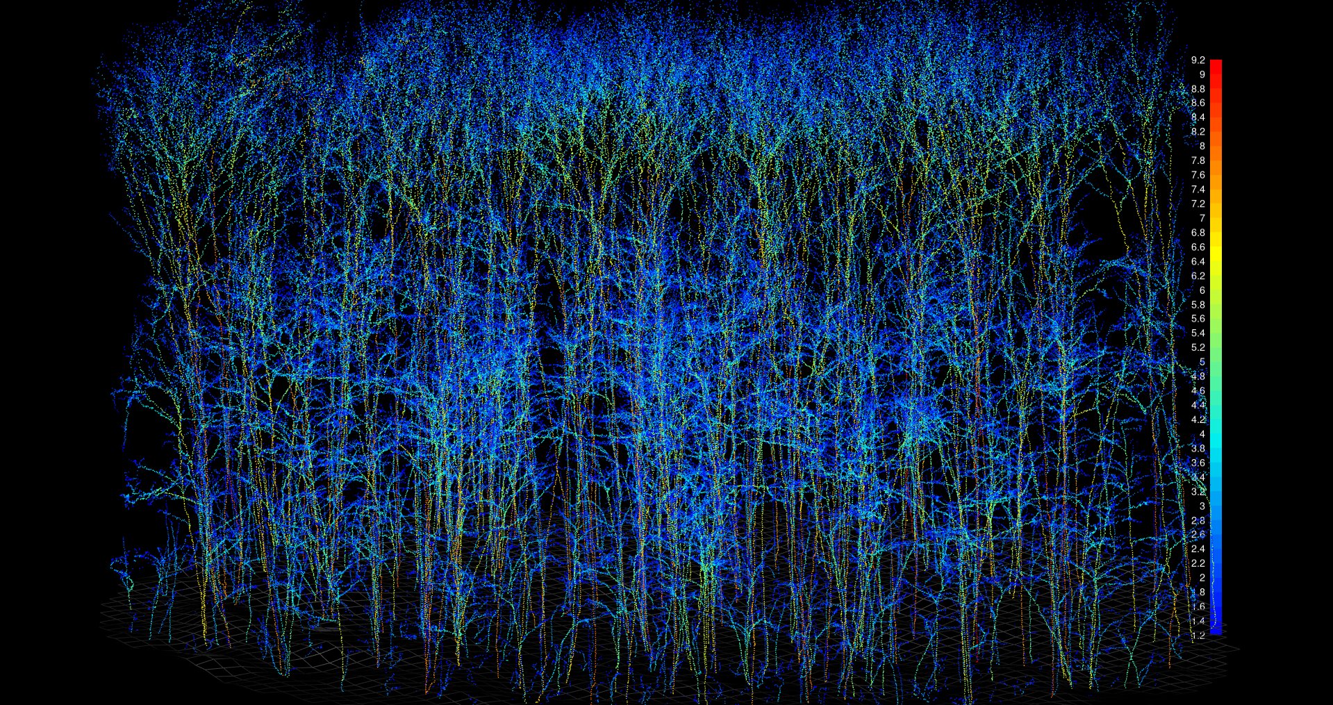
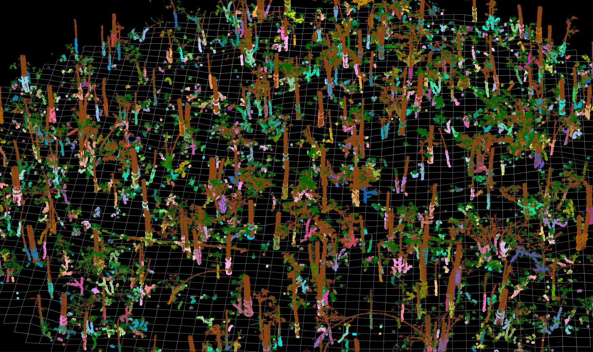
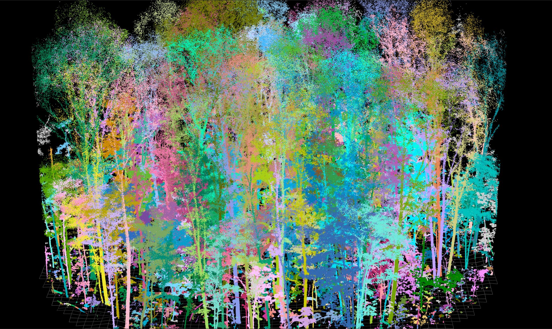
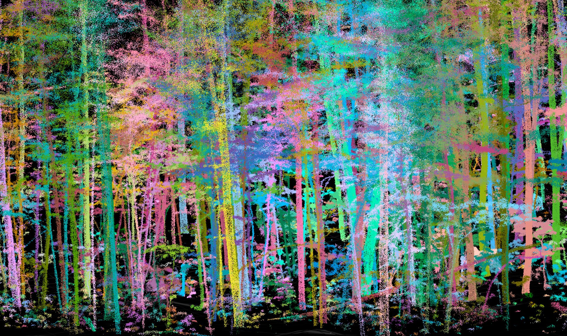
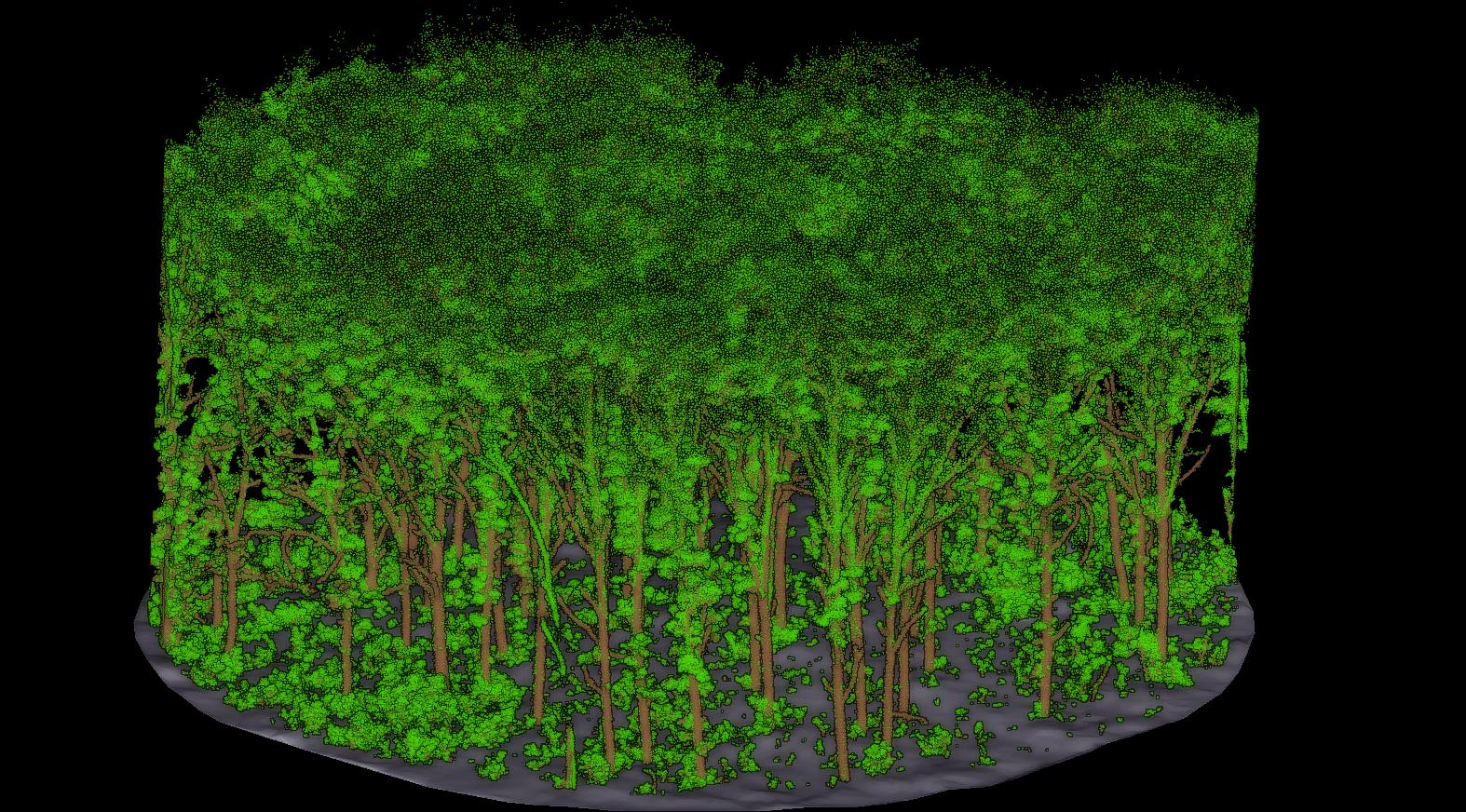
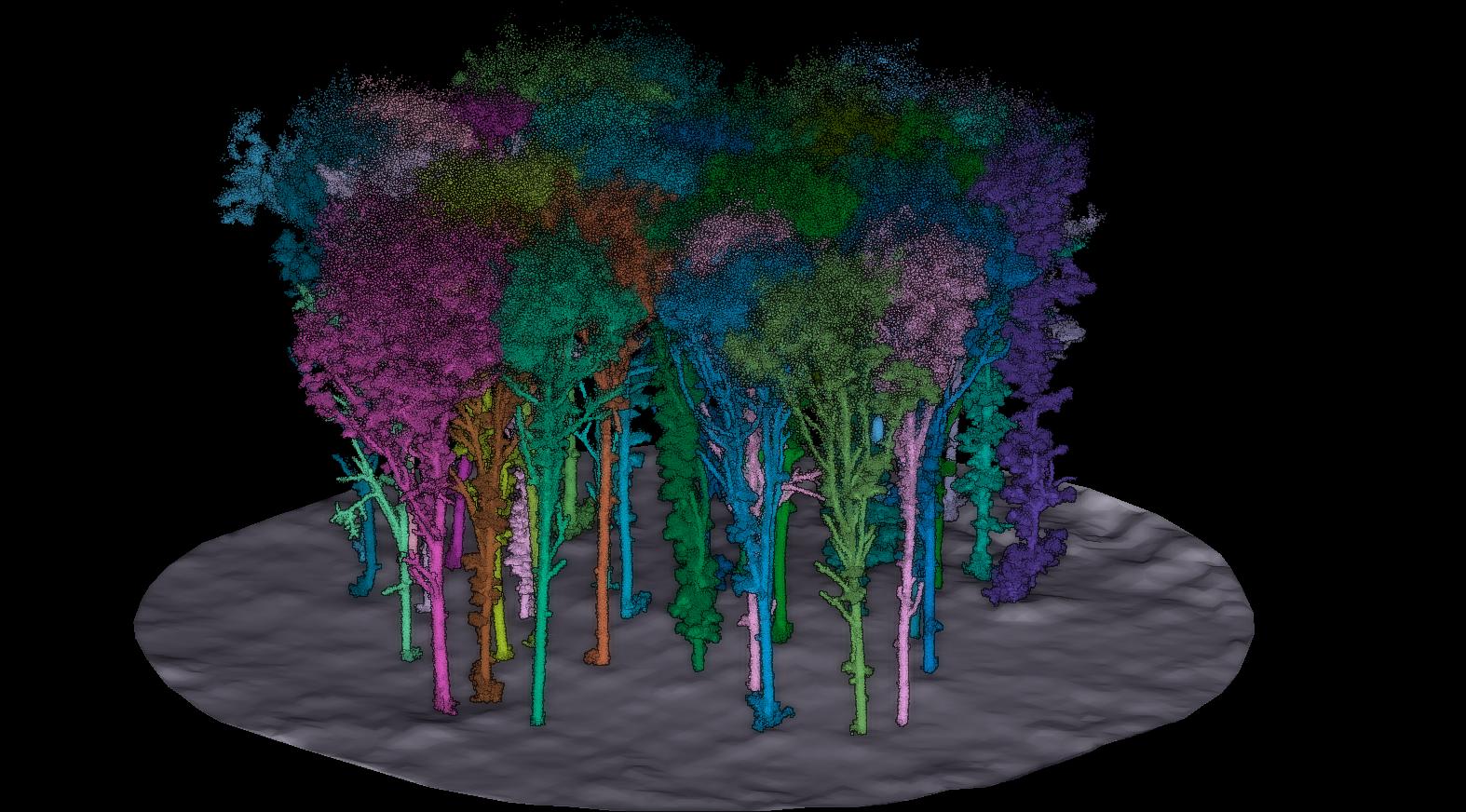
While sketches are useful for understanding and demonstrating the workflow, they do not capture the true complexity of real scenes. In particular, the workflow description presented so far is simplified. The following images show real data.

Passage points in a real scene. We have a lot of passage points.

Passage points close to the ground are the ones of interest. Green passage points are long paths from tall trees, while red passage points are short paths from bushes and low vegetation. Red circles are fitted on wood points (not described in previous sections) to make connected component merging more robust.

Passage points that are connected through wood points are assigned the same IDs.

Rendering of the first 2 m of the scene with semantic classification and the retained seeds.

Final instance segmentation. Wide view.

Final instance segmentation. Close view.

6.4 Common mistakes

Overall, the approach gives very good results. Yet, the most common error (putting aside issues with lianas in tropical forests) that users may encounter in instance segmentation is over-segmented trees receiving two or more IDs instead of one. The occurrence of such errors ranges between 0 and 5 per 1,000 trees depending on scene complexity, with higher occurrences in TLS than MLS. The error is particularly prominent with massive buttress trees.

Arbor v1.1.0 (currently available in beta-testing in the development branch on github (devel)) introduced an over-segmentation solver module. Starting in v1.1.0, segment_instance() automatically detects and fixes a significant number of over-segmentation cases. The module is enabled by default and can be turned off (restoring v1.0.0 behavior) via:

arbor_parameters_default$instance$oversegmentation_solver_enabled = FALSE

If disabled at segmentation time, it can still be executed during post-processing on an already segmented point cloud using:

las <- resolve_oversegmentation(las)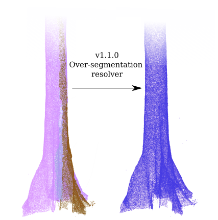

Arbor v1.0.0 tends to oversegment some trees, and especially tends to oversegment large buttress trees. v1.1.0 introduces an over-segmentation solver that significantly reduces the occurrence of such problems (which were already relatively rare).

6.5 Cleaning understory

At this stage, the scene is largely segmented. If everything went well, every tree, sapling, and bush has been segmented and assigned an ID. However, in practice, it is unrealistic to expect every tiny feature, such as small bushes or saplings, to be perfectly segmented. These features are extremely complex, interleaved, and noisy.

Moreover, they have virtually no significance in terms of carbon stock and are not harvested. Consequently, we suggest flagging all instances below a certain size threshold, typically 2 or 4 meters. The flagged trees won’t be processed in next steps.

Cleaning the understory is optional. You may keep all vegetation if desired.

las <- flag_small_trees(las, max_height = 2)

Note

Be careful, flag_small_trees() does not removes points. It assigns all small instances a UserData attribute value equal to the constant ARBORUNDERSTORY value. This saves memory and allows to easily revert the operation by calling again flag_small_trees() with another max_height parameter. To actually remove those points users can use las <- lidR::filter_poi(las, UserData != ARBORUNDERSTORY) but this is not necessary in Arbor.

Cleaned scene after removing small-size instances

6.6 Buffer Clipping and Edge Artifacts

Important

This section is of major importance. Please read it carefully.

A common issue with pathfinding is that we need to find a path to the ground. This becomes problematic at the edges of a dataset when the dataset has been clipped. At the edges, we alway have floating branches and trunks that are not connected to the ground. Consequently, the only path to reach the ground or a seed may be through a nearby tree.

The pathfinder can only reach the seeds of the nearby tree since the branches are not connected to the ground by another path.

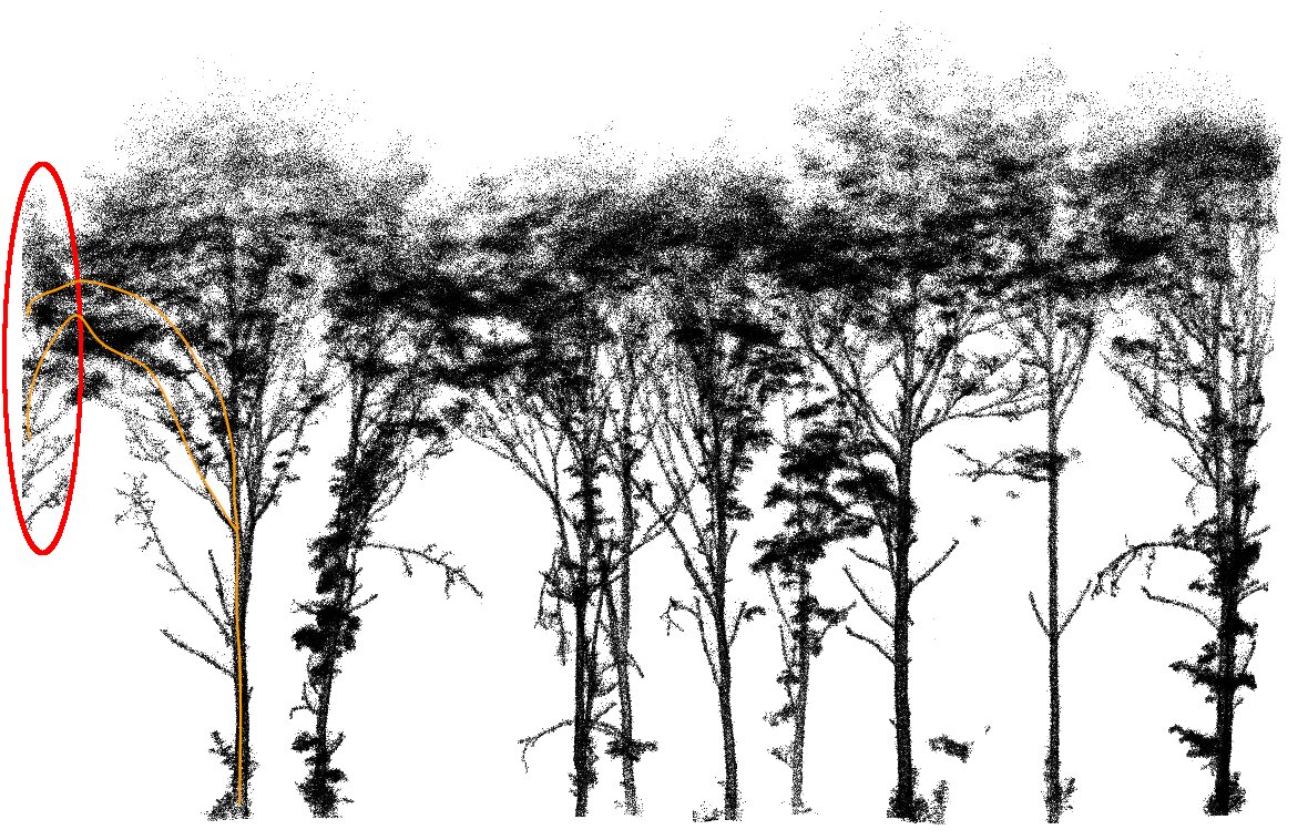
This produces invalid results, especially with large trees. Sometimes, for tilted trees, we may even see half of a trunk floating.

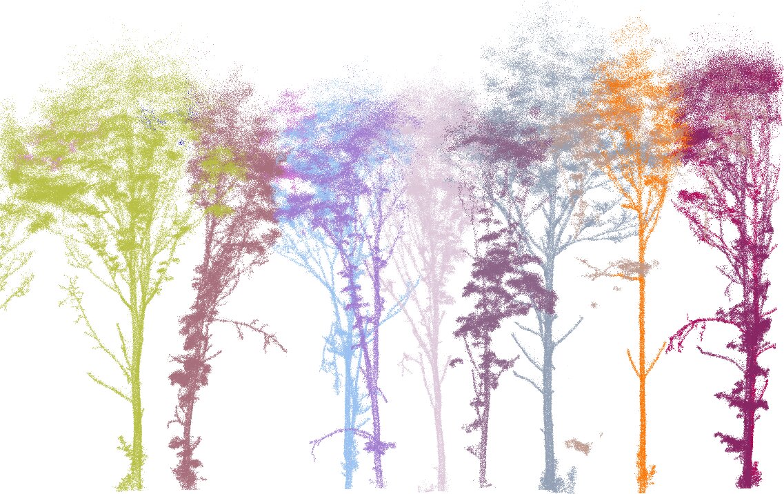
To avoid these issues, it is important to work with a scene larger than the area of interest, so that boundary trees can be removed (see also Section 2.1). In the images above, the green tree on the left and the reddish tree on the right should be removed. While the reddish tree may appear fine, this is merely coincidental: the scene happened to be cut just between two trees.

This can be achieved by flagging a buffer around the point cloud. The buffer size should correspond to the extent of the largest possible tree. Typically, we recommend a buffer of at least 10 meters, although this may vary depending on forest type and tree sizes. The flagged trees won’t be processed in next steps.

las <- flag_buffer(las, seeds, -10)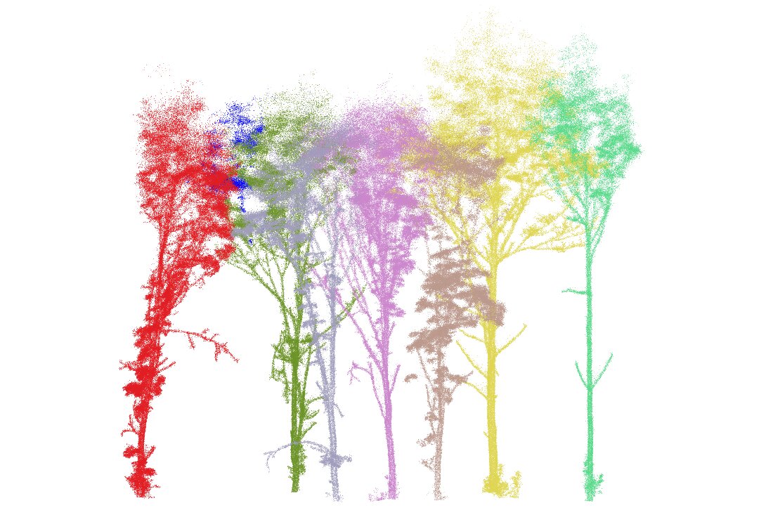

Edge trees were removed

Note

Be careful, flag_buffer() does not actually remove points. It assigns all instances in the buffer an attribute UserData with a constant equal to ARBORBUFFER. This saves memory and allows users to easily revert the operation by calling flag_buffer() a second time with another buffer value. To actually remove those points users can use las <- lidR::filter_poi(las, UserData != ARBORBUFFER) but this is not necessary in Arbor.

Visualization on real data:

6.7 Rendering & Filtering

The function plot_instance() renders the instance segmentation. All points have an attribute treeID. A treeID = 0 is equivalent to NA. Valid instances are guaranteed to not have a treeID equal to 0. Only strictly positive ID are valid.

Users can filter out valid tree with las <- lidR::filter_poi(las, UserData == ARBORTREE).

The function colorize_tree() adds RGB colors to the point cloud for rendering in external softwares.

6.8 Parameters

Arbor is designed to be parameter-free. Most internal parameters are intentionally undocumented, as they require a deep understanding of the internal pathfinder and are not meant for routine tuning.

Two parameters, however, can be safely adjusted to improve connectivity in sparse point clouds:

params$path_finder$k_neighborhood_connectivity
params$path_finder$max_gap

• k_neighborhood_connectivity defines the number of neighbors used to build the graph (default: 10).
• max_gap defines the maximum allowed distance between connected points (default: 1 m).

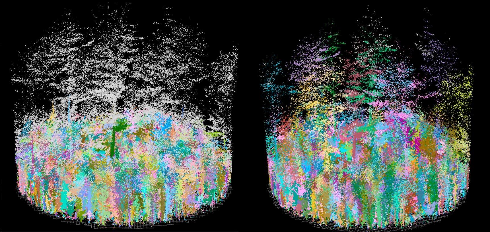
In sparse canopies, especially near tree tops, default values may fail to connect upper part or apexes to lower sections. Increasing these values can improve graph connectivity. However, this is rarely necessary, as internal safeguard routines are already implemented to maintain good connectivity in sparse regions.

Multilayered plot with extremely sparse sampling in upper canopy layers without the automatic connectivity fix (left) and with the automatic connectivity fix enabled (right).

Important

Changing these parameters also requires recomputing semantic segmentation, since it relies on the same pathfinder.

6.9 Point-wise Classification Accuracy

Is the instance semantic classification accurate? In practice, the answer here mirrors the case of semantic segmentation, and for the same reasons.

Point-wise classification accuracy is not a meaningful indicator of overall system performance. Even if our algorithm achieves 95–99% accuracy at the point level, this tells us very little about the practical quality of the final output. The remaining 1% of points, especially if they occur on tree boundaries or in areas critical for mensuration, can significantly distort measurements. Even a model that is 99.9% accurate could still produce unacceptable results if the remaining 0.1% introduces systematic or structurally important errors.

What truly matters is not how many points are classified correctly, but whether the segmentation produces coherent, reliable instances. For our application, this means accurately identifying individual trees and correctly estimating their position, DBH, height, and volume. These are the metrics that matter, and these are the ones we validate and discuss later.

For this reason, point-wise classification accuracy provides almost no practical insight.

6.10 Code

6.10.1 Function List

• find_seeds()
• segment_instance()
• plot_instance() : render the instance segmentation
• flag_small_trees()
• flag_buffer()
• plot_semantic_instance() : render the instance + semantic segmentation
• colorize_tree(): adds RGB colors to the point cloud for rendering in external softwares

6.10.2 Full Code

library(lidR)
library(arbor)

params <- arbor_parameters_default
params$global$cut_above_ground = 0.25
filter <- "-keep_random_fraction 0.25"

las <- readTLS(file, select = "xyz", filter = filter)

las <- hybrid_homogeneization(las)
las <- segment_ground(las)
las <- wood_likelihood(las, params)
las <- segment_semantic(las, params)
see <- find_seeds(las, params)
las <- segment_instance(las, see, params)
las <- flag_small_trees(las, max_height = 2)
las <- flag_buffer(las, see, -10)