3  Data Decimation

3.1 Summary

Ground-based laser scanners (MLS, TLS) produce point clouds that are heavy, noisy, and unevenly sampled, the worst combination for point cloud processing. To make computation feasible and results consistent, we need to aggressively decimate our data before any analysis.

Note

TL;DR: The main message of this chapter is: use our decimation process. Do not apply 1 cm voxel decimation, and do not process the full point cloud.

3.2 Why Decimate at All?

Three reasons drive aggressive decimation:

1. Computability: reduce RAM consumption to avoid overflow.
2. Speed: keep runtimes in the range of minutes on a laptop.
3. Consistency: most point cloud algorithms are sensitive to local density. Bringing every dataset to the same target density eliminates the need to re-tune parameters per dataset. Arbor is parameterless because every dataset is prepared in the same way, resulting in a roughly conform point spacing

The third point is often overlooked but is of major importance.

3.2.1 More Points Is Not More Accuracy

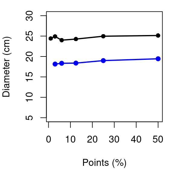
This is counter-intuitive but important: more points does not means more accuracy but it’s definitely synonymous with runtime blow-up and crazy RAM consumption. The figure below shows trunk slices at various decimation levels: from 50% down to 1% of the original point cloud.

10 cm slice at breast height, subsampled from 50% to 1% of the original point cloud.

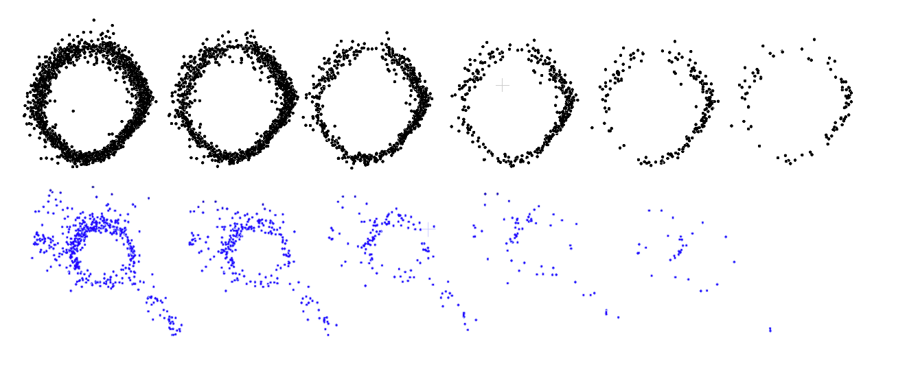
Using RANSAC circle fitting, measured tree diameter remains stable from the full point cloud all the way down to 99% decimation. One percent of the points is still sufficient to measure a tree reliably.

DBH measured as a function of decimation. The percentages correspond to the proportion of points remaining after subsampling.

This holds because MLS sensors cannot locate a target within better than 2 or 4 cm. Additional points carry no new information, only redundancy. Redundancy is expensive in storage and computation.

This confirms that we don’t need an indecent amount of points to process ground-based point clouds and make reliable measurements with proper methods. Even 1% of the points is sufficient to measure a tree! That said, we do not process just 1% of the data. Upper canopy points are far sparser than trunk points, so we typically retain 20–30% of the original cloud, around 25% for MLS and up to 50% for TLS, to preserve enough detail throughout the full vertical profile.

3.3 Choosing a Decimation Method

Three main options exist: random, voxel, and Poisson sampling.

3.3.1 Random Sampling

Random sampling is non-spatial: it removes points uniformly at random, preserving the original density distribution, including its noise. Isolated noise points have the same chance of being discarded as any other point. The signal-to-noise ratio is therefore unchanged after random decimation. This is a desirable property.

Its weakness: it cannot homogenize an unevenly sampled point cloud preserving the huge vertical variations.

3.3.2 Spatial Sampling (Voxel and Poisson)

Spatial sampling methods, on the other hand, homogenizes point spacing. Unlike random sampling an isolated noise point as 100% chance to be retained. If there is an isolated noise point somewhere, it will be retained by construction. Spatial methods are excellent at homogenizing the point cloud and preserving poorly sampled details, but they also amplify noise by design.

That last property is also their flaw: spatial sampling amplifies noise, which is exactly what we cannot afford.

3.3.3 Spatial vs. Random

In Arbor, we are capable of segmenting very small branches and saplings lost in the noise that are geometrically undetectable (e.g., too small and too noisy to fit any cylinder). To do so, we track local high densities. In order to track local high density, we need to preserve these local density variations. However, a weakness of spatial sampling is that it can easily loose density variations.

In Arbor, we can perfectly segment some tiny saplings or small branch segments based on locally high-density tracking.

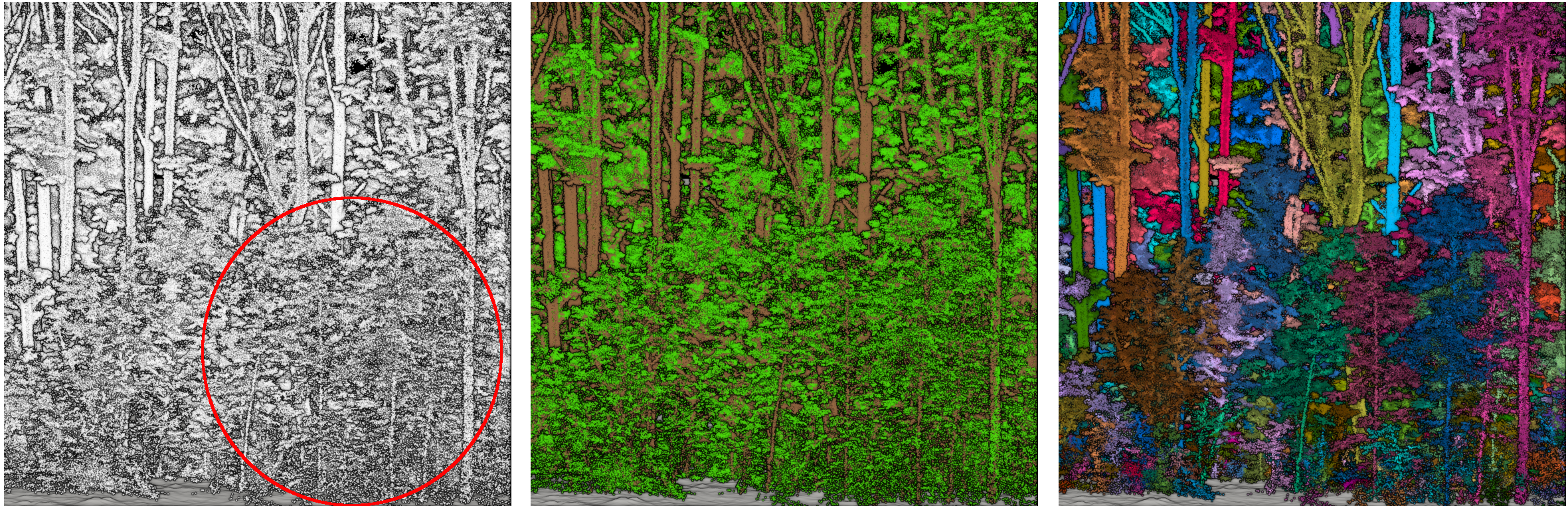
To compare we created a semi-realistic simulation of a tiny branch in a noisy foliage below. Visually in the raw point cloud, we are able to detect and track the branch based on local density variations. After random sampling (70% of points removed), the branch is still clearly present in the point cloud. After spatial sampling (only ~50% of points removed), the branch’s existence is far less obvious, and the data-to-noise ratio has increased significantly.

From left to right: raw data, random sampling (removing 70%), voxel sampling (removing 50%), and Poisson sampling (removing 50%), demonstrating how spatial sampling can amplify noise.

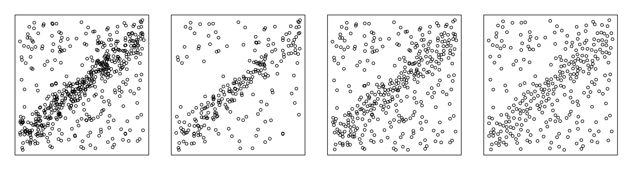
Ultimately, it is very easy to completely lose a feature with spatial sampling, whereas it is essentially impossible with random sampling, because the noise ratio remains stable. The simulated figures below are close to what really happens within the foliage. Applying a spatial sampling retains all the noisy foliage points while loosing some details in branches (which are already not detailed at all).

From left to right: raw data, random sampling, voxel sampling, and Poisson sampling, demonstrating how easily features can be lost through spatial sampling and noise amplification.

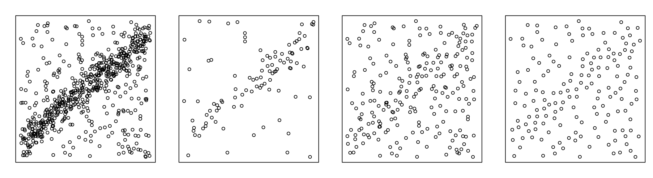
This is a serious problem of spatial sampling no matter which method is used (the worst being to retain the center of the voxel as a point). Arbor leverage local variations of density to track and disentangle branches that otherwise would not detectable with pure geometric analysis. We need to preserve density variation. Thus we need random sampling!

But spatial sampling also has advantages. We must weigh the pros and cons. The table below summarizes the trade-off:

Problem	Random Sampling	Spatial Sampling
Data reduction	✅	🔶 limited
Noise	🔶 neutral	❌ amplifies noise
Homogenization	🔶 no effect	✅
Sparse region preservation	❌	✅

No single method solves all problems. We need both.

3.4 Our Hybrid Approach

We developed a hybrid approach. We do not claim it is the best solution, but it offers a practical trade-off that:

• works reasonably fast,
• provides decent results at the end of the pipeline,
• and performs consistently across datasets.

We combine three steps:

Step	Purpose
Random sampling	Aggressive data reduction at read time
Barycentric Voxel Decimation (BVD)	Homogenization without amplifying noise
Random re-injection (~10%)	Restore local density variations

The idea is to first apply a random decimation at read time such as 70% of the point are not even loaded in memory

BVD differs from standard voxel decimation: instead of keeping a random point per voxel or worse, the voxel center, it retains the point closest to the barycenter of all points within the voxel i.e., the point located where local density is highest. This achieves homogenization while limiting the noise amplification that makes standard spatial sampling problematic. We call it density-preserving spatial sampling.

The final re-injection step brings back a small fraction of discarded points to recover density variation that BVD have smoothed away.

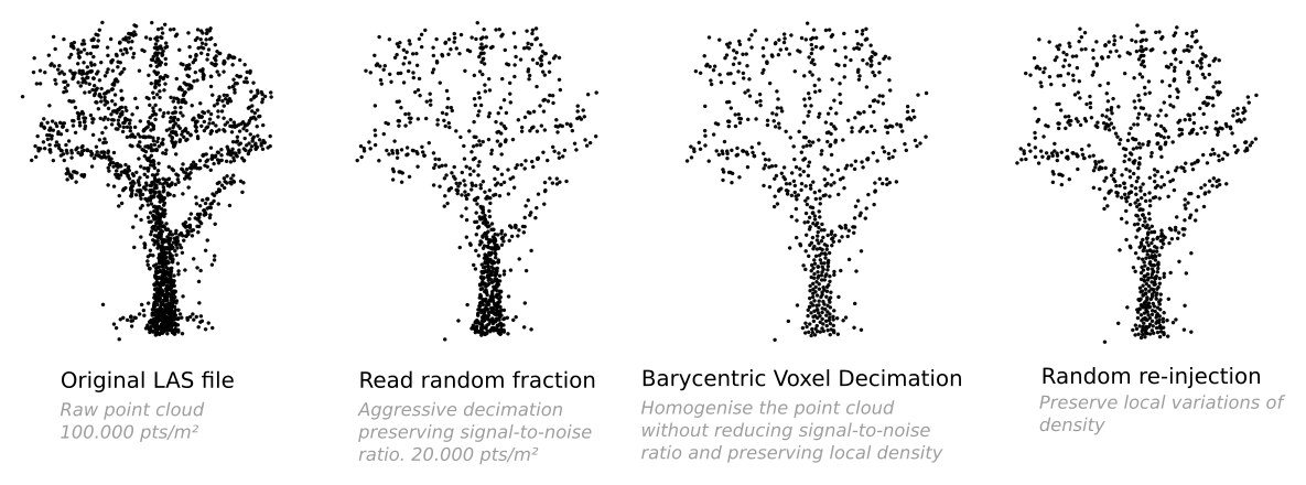
This pipeline is a practical compromise, not a perfect solution. It is fast enough to run on full MLS datasets, produces consistent results, and avoids the noise amplification that disqualifies pure spatial sampling.

3.5 Data Loading

This brings us to the first line of code for loading the data:

las <- readTLS(file, select = "xyz", filter= "-keep_random_fraction 0.25")
las <- hybrid_homogeneization(las)

Using readTLS() is recommended. It sorts the point cloud so that points that are spatially close are also stored close together in memory. This significantly improves computation time by reducing L1 cache misses and pointer indirection (technical details appreciated by computer enthusiasts).

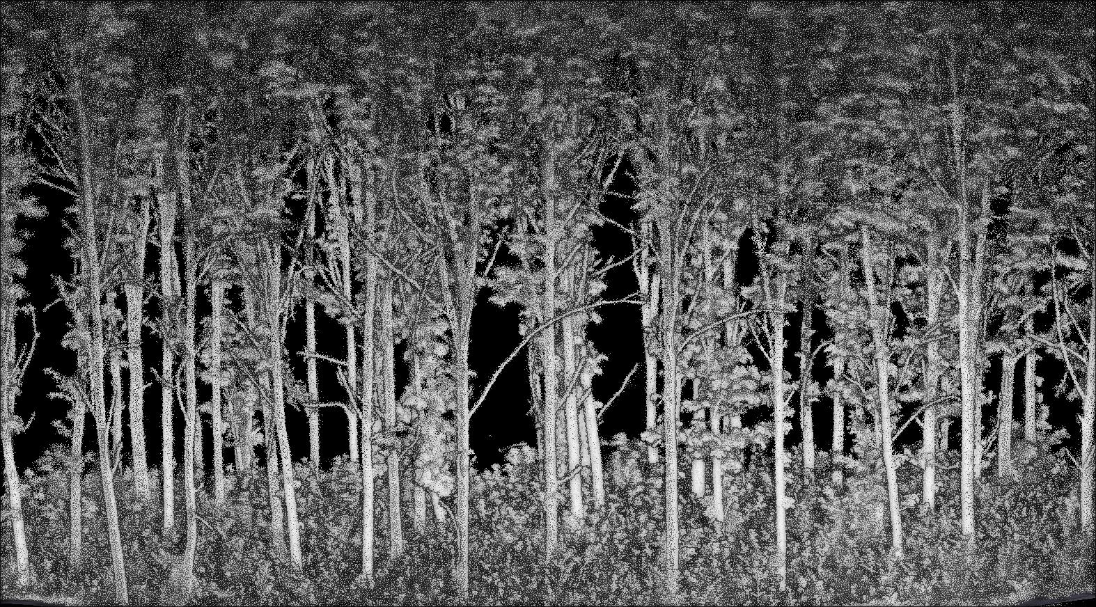
The fraction of points to retain depends on the original point cloud, but 25% is a good starting point. The function hybrid_homogeneization() then aims to homogenize the data as effectively as possible. When the forest is well sampled up to the canopy top, we can be more aggressive and discard more points. However, if the scene suffers from very low sampling near the apexes, it may be better to retain more points before applying spatial sampling. Remember, no solution is perfect, all are trade-offs.

3.6 Our Recommendations

Loading only 25% of a point cloud still means storing 75% of unnecessary data. It also requires reading and decompressing gigabytes of data for nothing, which is both time-consuming and cumbersome.

We recommend randomly decimating the original point cloud by 50% into a new file, then deleting the original file (since it will likely never be processable anyway) and working only with the pre-decimated file.

By subsequently reading only 40-50% of this pre-decimated file, you can significantly reduce storage requirements and processing time.

3.7 Code

3.7.1 Function List

• readTLS(): read LAS/LAZ file and perform on-the-fly random decimation without loading any useless point in memory
• hybrid_homogeneization(): performs a custom homogenization with re-injection of random points to preserve local variations of density

3.7.2 Full Code

library(lidR)
library(arbor)

params <- arbor_parameters_default
filter <- "-keep_random_fraction 0.25"

las <- readTLS(file, select = "xyz", filter = filter)
las <- hybrid_homogeneization(las)